What Is Gradient Descent? Definition, Formula and Examples

By Dr. Zubair Khalid, DVM, MS, PhD · 2026-10-03

Gradient descent is an iterative optimization algorithm that finds the parameter values which produce the lowest value of a loss function. It starts from an initial guess, measures the slope of the loss at that point, and takes a small step in the downhill direction. Repeating this process many times moves the parameters toward a minimum.

Quick Answer

Gradient descent minimizes a loss function by repeatedly updating parameters in the direction that reduces loss.
The update rule is $w \leftarrow w - \eta \nabla L(w)$, where $\eta$ is the learning rate and $\nabla L(w)$ is the gradient.
The gradient points uphill, so you subtract it to move downhill.
The learning rate controls step size. Too large and the process can overshoot, too small and it converges slowly.
It is the most common optimization algorithm in machine learning and deep learning [1].

What Gradient Descent Means

In plain terms, gradient descent is a way of finding the bottom of a curve when you cannot solve for it directly. You feel the slope under your feet and step downhill. Each step is small, and after enough steps you are close to the lowest point.

The precise definition: gradient descent is a first-order iterative optimization algorithm for finding a local minimum of a differentiable function. It uses only the first derivative (the gradient) when updating parameters, and the stepwise process moves downhill toward a local minimum [1]. For a linear regression model, it is the technique that iteratively finds the weights and bias that produce the model with the lowest loss [2].

The word "gradient" is the key. For a function of one variable, the gradient is just the derivative. For a function of many variables, the gradient is a vector of partial derivatives, one per parameter. It points in the direction of steepest increase, so its negative points in the direction of steepest decrease.

How It Works

The core update for a single parameter is:

$$w_{k+1} = w_k - \eta \nabla f(w_k)$$

Each symbol means the following.

Symbol	Meaning
$w_k$	The parameter value at step $k$
$w_{k+1}$	The updated parameter value
$\eta$	The learning rate, a small positive number that controls step size
$\nabla f(w_k)$	The gradient of the objective at the current parameter value

The algorithm repeats four steps until it stops improving: calculate the loss with the current parameters, determine the direction that reduces loss, move the parameters a small amount in that direction, then repeat [2]. Training usually begins with randomized weights and biases near zero [2].

For a linear model $y = wx + b$ trained with mean squared error, the two gradients are:

$$\frac{\partial L}{\partial w} = \frac{2}{n}\sum_{i=1}^{n}(\hat{y}_i - y_i)x_i \qquad \frac{\partial L}{\partial b} = \frac{2}{n}\sum_{i=1}^{n}(\hat{y}_i - y_i)$$

Here $n$ is the number of observations, $\hat{y}_i$ is the predicted value, and $y_i$ is the actual value. The factor of 2 comes from differentiating the squared error. Both gradients are linear functions of the parameters, which is why the loss surface for linear regression is a bowl shape with a single minimum [3].

Worked Example

The dataset is study hours versus exam scores for 10 students.

Hours	Score
1	45
2	52
3	58
4	63
5	68
6	74
7	79
8	85
9	90
10	96

The model is $\hat{y} = wx + b$, initialized at $w = 0$ and $b = 0$. The loss is mean squared error, $L = \frac{1}{n}\sum(\hat{y} - y)^2$. The update rule uses a learning rate of 0.01:

$$w \leftarrow w - 0.01 \cdot \frac{\partial L}{\partial w} \qquad b \leftarrow b - 0.01 \cdot \frac{\partial L}{\partial b}$$

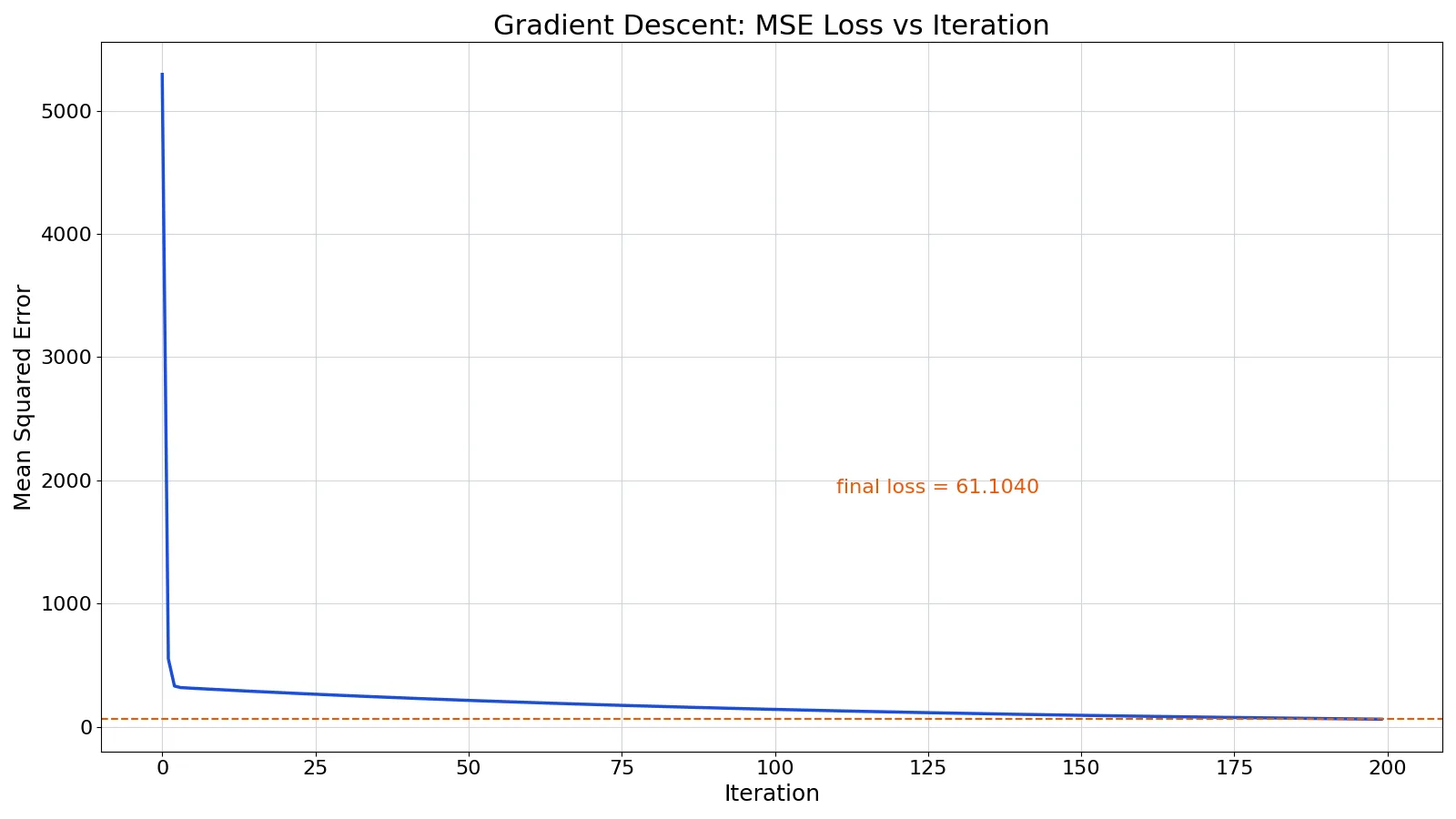
At iteration 0, with both parameters at zero, every prediction is 0 and the loss is 5294.4000. That is a large error because the model predicts a score of zero for every student.

The gradient with respect to $w$ at that point is large and negative, because the errors $(\hat{y} - y)$ are all negative and the hours are all positive. Subtracting a negative number increases $w$. The gradient with respect to $b$ is also negative, so $b$ increases too. After the first update, the line has already tilted upward and shifted up.

Each subsequent iteration recomputes the predictions, the errors, the two gradients, and the two parameters. The loss falls quickly at first, then more slowly as the parameters approach the minimum. After 200 iterations the loss is 61.1040, with learned values $w = 7.9497$ and $b = 23.7531$. These values have not converged yet. The least squares solution is $w = 5.5394$ and $b = 40.5333$, with a loss of 0.2497, and this learning rate needs a few thousand iterations to reach it, so the slope of 7.95 should not be read as the effect of an extra study hour.

import numpy as np
x = np.array([1,2,3,4,5,6,7,8,9,10], dtype=float)
y = np.array([45,52,58,63,68,74,79,85,90,96], dtype=float)
w, b, lr = 0.0, 0.0, 0.01
for i in range(200):
    yp = w*x + b
    e = yp - y
    loss = np.mean(e**2)
    w -= lr * (2/len(x)) * np.sum(e*x)
    b -= lr * (2/len(x)) * np.sum(e)
print(round(loss, 4))  # 61.1040

Output:

61.1040

The loss curve drops from 5294.4000 to 61.1040 over 200 iterations. The shape of that curve, steep at the start and flattening near the end, is typical. The model has converged when the loss stops falling, which for linear models means it has reached the lowest possible loss [2]. This run has not reached that point, because the loss is still falling by about 0.5 per iteration at iteration 200 and the lowest possible loss is 0.2497.

How to Interpret It

The loss value tells you how well the current parameters fit the data. A loss of 61.1040 for this dataset means the average squared prediction error is about 61, so the typical prediction is off by roughly 8 points. That is a poor fit for data this close to a straight line, where the best possible loss is 0.2497, and it shows the run stopped too early.

The learned parameters are the output you actually use. Once training has converged, the slope $w$ (5.5394 for this dataset) is the estimated change in score per additional hour, and the intercept $b$ (40.5333) is the predicted score at zero hours, which may or may not be meaningful depending on the context. If you want to understand how a slope is read in a regression setting, see What Is Slope? Definition, Formula and Regression Examples.

Watch the loss curve, not just the final number. A curve that falls smoothly and flattens suggests a healthy run. A curve that bounces or rises suggests the learning rate is too high. A curve that is still falling steeply at the last iteration suggests you stopped too early.

When to Use It (and when not to)

Use gradient descent when the loss function is differentiable and you cannot solve for the minimum in closed form. This covers most of machine learning, including linear regression, logistic regression, and neural networks [1]. It is also the natural choice when the dataset is too large to fit in memory, because you can estimate the gradient from a subset of the data.

Do not use it when a direct solution exists and is cheap. For ordinary least squares with a modest number of features, the normal equation gives the exact answer in one step. Gradient descent only approximates that answer, and it needs tuning.

Do not use it on non-differentiable objectives without care. Gradient descent can still work on functions with kinks, points where the derivative is undefined, because frameworks such as PyTorch use a fixed one-sided derivative at those points, which is why functions like ReLU are usable in deep networks [4]. But the behavior is not guaranteed.

Gradient Descent vs Stochastic Gradient Descent

Stochastic gradient descent (SGD) is a variant that estimates the gradient from a randomly sampled batch of training data instead of the full dataset [4]. The full-batch version computes the exact gradient but is slower per step. SGD computes a noisy estimate but takes many more steps per unit of time.

Aspect	Batch gradient descent	Stochastic gradient descent
Gradient source	All training examples	A random subset (batch)
Cost per step	High	Low
Gradient accuracy	Exact	Approximate
Path to minimum	Smooth	Noisy
Best for	Smaller datasets	Large datasets

The tradeoff is accuracy against speed, and the batch size is the hyperparameter that controls it [4]. A batch almost as large as the full dataset gives an estimate close to the true gradient. A small batch is faster but less accurate [4].

Common Mistakes

Setting the learning rate too high. The loss can oscillate or grow instead of falling. Fix: reduce the learning rate and rerun, or use a decaying schedule.
Setting the learning rate too low. Training takes far more iterations than needed. Fix: increase it gradually and watch the loss curve.
Forgetting to scale features. Parameters on very different scales need very different step sizes. Fix: standardize inputs before training.
Stopping too early. A loss still falling at the last iteration means the model is undertrained. Fix: run more iterations or check convergence.
Confusing the gradient sign. The gradient points uphill, so you subtract it. Adding it moves you away from the minimum.
Assuming the minimum is global. For non-convex functions, gradient descent can settle at a local minimum or a flat point [5].

Limitations

Gradient descent finds a point where the gradient is close to zero, and that point is not always a minimum. For non-convex functions it can converge to a local minimum, and it can also stagnate at a point that is neither a minimum nor a maximum [5]. There are even convex functions with no minimum at all, such as $f(x) = \exp(-x)$, where gradient descent with a positive learning rate diverges toward infinity [5].

The method also says nothing about model quality on its own. It minimizes whatever loss you give it, so a poorly chosen loss produces a poorly chosen model. Gradient descent does not select the loss function and does not change the dataset [2]. It only finds the parameters that minimize the loss you defined.

Frequently Asked Questions

What is the difference between gradient descent and gradient learning?

Gradient learning is an informal term people use for the same idea: learning model parameters by following gradients. Gradient descent is the standard, precise name for the algorithm. If you see "gradient learning" in a search, it almost always refers to gradient descent or to gradient-based learning algorithms in general [4].

Why do you subtract the gradient instead of adding it?

The gradient points in the direction of steepest increase of the function. To reduce the loss, you move in the opposite direction, so you subtract. The update $w_{k+1} = w_k - \eta \nabla f(w_k)$ encodes exactly that [1].

How do I choose the learning rate?

Start with a small value and watch the loss curve. If the loss falls smoothly and flattens, the rate is reasonable. If it bounces or grows, lower it. If it falls very slowly, raise it. Many libraries also offer adaptive schedules, where the learning rate starts higher and decays over time [6].

Does gradient descent always find the best solution?

No. For convex loss functions such as mean squared error in linear regression, it converges to the global minimum [2]. For non-convex functions, it can get stuck at a local minimum or a flat point where the gradient is zero but the point is not a minimum [5].

What is the difference between batch and stochastic gradient descent?

Batch gradient descent uses all training examples to compute each gradient update. Stochastic gradient descent uses a randomly sampled subset, which makes each step cheaper but noisier [4]. The scikit-learn SGD implementations use this approach and let you control the learning rate schedule [6].