Eigenvalues and Eigenvectors: Definition and Examples

By Dr. Zubair Khalid, DVM, MS, PhD · 2026-10-03

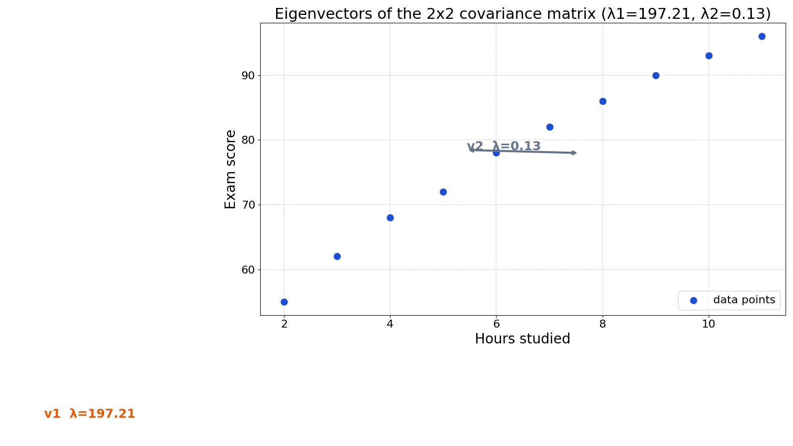
Eigenvectors are the special directions that a matrix only stretches, never rotates. The amount of stretch along each of those directions is the matching eigenvalue. This article defines both terms, shows how they are computed, and works through a real example using a covariance matrix from 10 students' study hours and exam scores.

Quick Answer

An eigenvector of a square matrix $A$ is a nonzero vector $v$ where $Av = \lambda v$ for some scalar $\lambda$ [1][2].
The scalar $\lambda$ is the eigenvalue, sometimes called the characteristic value [3].
Geometrically, multiplying by $A$ changes the length of an eigenvector but not its direction [2].
Eigenvalues are found by solving the characteristic equation $\det(A - \lambda I) = 0$ [3][4].
In data analysis, eigenvectors of a covariance or correlation matrix give the directions of maximum variance, which is the basis of principal component analysis [5][4].

What Eigenvectors and Eigenvalues Mean

In plain terms, imagine pushing on a rubber sheet. Most points move sideways as well as outward. A few special directions only stretch or shrink. Those directions are the eigenvectors, and how much they stretch is the eigenvalue.

The precise definition: for a square matrix $A$, a nonzero vector $v$ is an eigenvector if there is a scalar $\lambda$ such that

$$Av = \lambda v$$

The scalar $\lambda$ is the eigenvalue associated with $v$ [1][2]. The word "nonzero" matters. The zero vector satisfies the equation trivially for any $\lambda$, so it is excluded by definition.

A matrix can have several eigenvalues, and each one comes with its own eigenvector. Eigenvalues can be real or complex, and an $n \times n$ real matrix can have complex eigenvalues [5]. Eigenvectors with distinct eigenvalues are linearly independent of each other [1].

How It Works

The equation $Av = \lambda v$ can be rewritten as $(A - \lambda I)v = 0$, where $I$ is the identity matrix. For a nonzero $v$ to solve this, the matrix $A - \lambda I$ must be singular, meaning its determinant is zero [3][4]:

$$\det(A - \lambda I) = 0$$

This is the characteristic equation. Solving it gives the eigenvalues. Here is what each symbol means:

Symbol	Meaning
$A$	The square matrix you are analyzing
$v$	An eigenvector of $A$, a nonzero column vector
$\lambda$	The eigenvalue paired with $v$
$I$	The identity matrix, same size as $A$
$\det$	The determinant of a matrix

For a $2 \times 2$ matrix, the characteristic equation is a quadratic, so you get two eigenvalues. For an $n \times n$ matrix, you get a polynomial of degree $n$ and up to $n$ eigenvalues [3].

Once you have an eigenvalue, substitute it back into $(A - \lambda I)v = 0$ and solve for $v$. The equations you get are always redundant, so you choose one component freely and the rest follow [6]. That freedom means eigenvectors are not unique. Any nonzero multiple of an eigenvector is still an eigenvector for the same eigenvalue, and only the ratio of the components is fixed [3][6].

Two checks are always worth running. The eigenvalues sum to the trace of the matrix, and they multiply to its determinant [4].

Worked Example

The dataset below records hours studied and exam score for 10 students. We build the $2 \times 2$ covariance matrix and find its eigenvalues and eigenvectors.

hours_studied	exam_score
2	55
3	62
4	68
5	72
6	78
7	82
8	86
9	90
10	93
11	96

Step by step:

Sample size: $n = 10$.
Mean hours studied: $\bar{x} = 6.5000$.
Mean exam score: $\bar{y} = 78.2000$.
Sample variance of hours: $\text{var}_x = 9.1667$.
Sample variance of score: $\text{var}_y = 188.1778$.
Sample covariance: $\text{cov}_{xy} = 41.2222$.
Covariance matrix: $C = \begin{bmatrix} 9.1667 & 41.2222 \\ 41.2222 & 188.1778 \end{bmatrix}$.
Characteristic equation: $\lambda^2 - 197.3444\lambda + 25.6914 = 0$.
Larger eigenvalue: $\lambda_1 = 197.2142$.
Smaller eigenvalue: $\lambda_2 = 0.1303$.
Unit eigenvector for $\lambda_1$: $v_1 = [-0.2141, -0.9768]$.
Unit eigenvector for $\lambda_2$: $v_2 = [-0.9768, 0.2141]$.
Trace check: $197.2142 + 0.1303 = 197.3444$, matching the trace.
Determinant check: $197.2142 \times 0.1303 = 25.6914$, matching the determinant.
Variance of the data projected onto $v_1$: $197.2142$.
Fraction of variance explained by $v_1$: $0.9993$.

The code that produces these numbers:

import numpy as np
X = np.array([[2,55],[3,62],[4,68],[5,72],[6,78],
              [7,82],[8,86],[9,90],[10,93],[11,96]], dtype=float)
C = np.cov(X, rowvar=False, ddof=1)
vals, vecs = np.linalg.eig(C)
print(vals)   # [0.1303 197.2142] (eig does not sort)
print(vecs)

Output:

eigenvalues = [0.1303 197.2142]
eigenvectors (columns) = [[-0.9768 -0.2141]
                          [ 0.2141 -0.9768]]

The eig function in numpy.linalg is the standard way to solve this problem in Python [7]. Note that the eigenvectors come back as columns, not rows, and that eig does not sort the eigenvalues, so sort them yourself before labeling $\lambda_1$ and $\lambda_2$.

How to Interpret It

The first eigenvector $v_1 = [-0.2141, -0.9768]$ points mostly along the exam score axis. The second, $v_2 = [-0.9768, 0.2141]$, points mostly along the hours axis. Because the two vectors are perpendicular, they form a new set of axes rotated relative to the original ones.

The eigenvalue $\lambda_1 = 197.2142$ is the variance of the data after projecting it onto $v_1$. That is the largest variance any single direction can capture. The second eigenvalue, $0.1303$, is tiny by comparison, so $v_2$ captures almost no spread.

The ratio $\lambda_1 / (\lambda_1 + \lambda_2) = 0.9993$ means the first direction explains 99.9% of the total variance. In practice, you could describe this dataset with one number per student instead of two and lose almost nothing. That reduction is exactly what principal component analysis does, and it is why eigenstructure figures heavily in multivariate procedures [4].

The signs of the eigenvector components are arbitrary. Flipping both signs of $v_1$ gives an equally valid eigenvector, because only the direction matters [3]. When you compare eigenvectors across software packages, check the direction, not the sign.

When to Use It (and when not to)

Use eigenvalues and eigenvectors when you want to find the dominant directions in a set of variables. Common cases include dimensionality reduction with PCA, understanding the shape of a covariance matrix, and detecting near-dependence between variables. If two variables are almost collinear, the smaller eigenvalue of the covariance matrix will be close to zero, which is a useful diagnostic when you check for multicollinearity.

Do not use them when your matrix is not square. Eigenvalues are defined only for square matrices. Do not use them on raw data without thinking about scale. If one variable is measured in thousands and another in single digits, the covariance matrix will be dominated by the large-scale variable, and the first eigenvector will mostly reflect that. Standardizing the variables first, which turns the covariance matrix into a correlation matrix, is often the better choice.

Also avoid reading too much into small eigenvalues. A near-zero eigenvalue can come from genuine redundancy, but it can also come from noise in a small sample.

Eigenvectors vs Singular Vectors

The closest related idea is the singular vector, which comes from singular value decomposition (SVD). The two are connected but not identical.

Property	Eigenvector	Singular vector
Defined for	Square matrices	Any matrix, including rectangular
Equation	$Av = \lambda v$	$Av = \sigma u$ and $A^T u = \sigma v$
Paired with	An eigenvalue $\lambda$	A singular value $\sigma$
Sign	Can be flipped freely	Can be flipped freely
Relationship	Eigenvectors of $A^T A$ are the right singular vectors of $A$	Singular values are the square roots of the eigenvalues of $A^T A$

For a symmetric matrix such as a covariance matrix, the two ideas nearly coincide. The eigenvectors of the covariance matrix are the right singular vectors of the centered data matrix, and the eigenvalues are the squared singular values divided by the degrees of freedom.

Common Mistakes

Thinking eigenvectors are unique. Any nonzero multiple of an eigenvector is also an eigenvector. The fix is to report unit-length eigenvectors or state the scaling you used [3].
Forgetting the nonzero condition. The zero vector is never an eigenvector, even though it satisfies the equation. The fix is to exclude it when you solve.
Reading eigenvectors as rows. In numpy.linalg.eig, the eigenvectors are the columns of the returned array. The fix is to check the shape and index accordingly [7].
Skipping the trace and determinant checks. These catch arithmetic errors fast. The fix is to verify that the eigenvalues sum to the trace and multiply to the determinant [4].
Running PCA on unstandardized variables. Variables with large units dominate the first component. The fix is to standardize when the scales differ.
Assuming every matrix is diagonalizable. A matrix with fewer than $n$ linearly independent eigenvectors is defective and cannot be diagonalized [5]. The fix is to check the number of independent eigenvectors before relying on a diagonal form.

Limitations

Eigenvalues and eigenvectors describe linear structure only. If the real relationship between your variables is curved, the leading eigenvector of the covariance matrix will still point somewhere, but that direction may not summarize the data well. A quadratic term or a different method may fit better.

Eigenvectors are also sensitive to the input matrix. Small changes in the data can rotate eigenvectors noticeably when two eigenvalues are close in size. In that situation, the individual directions are unstable even though the total variance they explain is not. Treat near-tied eigenvalues as a signal that the components should not be interpreted separately.

Frequently Asked Questions

What is the difference between an eigenvalue and an eigenvector?

An eigenvector is a direction that the matrix only stretches. An eigenvalue is the number that tells you how much stretching happens along that direction. They always come in pairs, one eigenvalue per eigenvector.

Can an eigenvalue be zero?

Yes. A zero eigenvalue means the matrix collapses that direction to nothing, which happens when the matrix is singular. In a covariance matrix, a zero eigenvalue means one variable is an exact linear combination of the others.

Why do eigenvectors matter in PCA?

PCA finds the eigenvectors of the covariance or correlation matrix and orders them by eigenvalue. The largest eigenvalue marks the direction with the most variance, so keeping only the top few eigenvectors compresses the data with minimal loss [5][4].

Do I need to normalize eigenvectors?

Not for the math, since any nonzero multiple works. For reporting and comparison, unit-length eigenvectors are the convention, and most software returns them that way by default [3][7].

How many eigenvalues does a matrix have?

An $n \times n$ matrix has exactly $n$ eigenvalues when you count repeated ones. Some may be complex, and some may repeat, which is why the multiplicity of an eigenvalue matters [5].