What Is Boosting? Definition and Examples for Analysts

By Dr. Zubair Khalid, DVM, MS, PhD · 2026-10-03

Boosting is an ensemble method that builds a strong predictive model by adding weak models one at a time, where each new model is trained to fix the mistakes of the model built so far [1]. It turns a classifier that is only slightly better than guessing into one that can be very accurate [2]. This article explains the definition, the mechanism, a worked example, and when boosting is the right choice.

Quick Answer

Boosting trains weak learners sequentially, not in parallel, and each learner focuses on the errors left by the previous ones [1].
The final prediction is a weighted sum of all the weak learners, so no single tree or stump decides the answer.
AdaBoost reweights misclassified training rows so later learners pay more attention to them [2].
Gradient boosting trains each new learner to predict the gradient of the loss, which for squared error is proportional to the signed error [3].
Shrinkage, also called the learning rate, scales each learner's contribution and controls how fast the model learns [1].

What Boosting Means

In plain terms, boosting means improving a weak model by committee, but a committee that meets in sequence. You start with a simple model, look at where it goes wrong, and add a second model whose job is to correct those specific errors. Repeat that a few hundred times and the combined model is far stronger than any single member.

The precise statistical definition: boosting is a stagewise additive modeling procedure. At each stage $t$ you fit a weak learner $h_t$ and update the current model

$$F_t(x) = F_{t-1}(x) + \alpha_t h_t(x)$$

where $\alpha_t$ is the weight given to that learner. The family includes AdaBoost, Gradient Boosting, LogitBoost, and many others [2]. Bickel, Ritov, and Zakai showed that the population version of the boosting algorithm converges to the Bayes classifier, which is the theoretically optimal decision rule [4]. That result is why boosting is treated as a principled statistical method and not just a practical trick.

How It Works

The mechanism differs slightly between the two best-known variants, but the skeleton is the same.

AdaBoost. Fit a weak learner on the training data. Compute its weighted error $err_t$. Set the learner's weight to

$$\alpha_t = 0.5 \ln\left(\frac{1 - err_t}{err_t}\right)$$

Then increase the weights on the rows that were misclassified and decrease the weights on the rows that were correct. The next learner sees a dataset where the hard cases matter more. A learner with error below 0.5 gets a positive weight, and a learner at exactly 0.5 gets zero weight because it carries no information.

Gradient boosting. Instead of reweighting rows, you fit each new weak model to the pseudo response, which is the error of the current strong model [1]. The update is

$$F_t(x) = F_{t-1}(x) + \eta \, h_t(x)$$

Here $\eta$ is the shrinkage or learning rate, and it scales down each tree's contribution [1]. A small $\eta$ means each tree moves the prediction only a little, so you need more trees but usually get a better fit. For regression with squared error loss, the gradient of the loss is proportional to the signed error, but that equivalence does not hold for other problem types, which is why gradient boosting uses the gradient of the loss directly [3]. Modern implementations use second-order information, the Hessian, in a variant called Newton boosting, which avoids the line-search step of ordinary gradient boosting [5].

The symbols, in one place:

Symbol	Meaning
$h_t(x)$	The weak learner fitted at stage $t$
$\alpha_t$	Weight assigned to learner $t$ in AdaBoost
$\eta$	Shrinkage or learning rate in gradient boosting
$F_t(x)$	The combined strong model after $t$ stages
$err_t$	Weighted error of learner $t$ on the training data

Worked Example

The dataset is a 60-row customer churn table with two features, tenure_months and monthly_charge, and a binary churn label. The first rows look like this.

tenure_months	monthly_charge	churn
2	70	1
20	25	0
3	73	1
21	27	0
4	76	1
22	29	0
5	79	1
23	31	0

The pattern continues: short tenures with high charges are labeled churn, longer tenures with low charges are not. The full table has 60 rows.

The steps, with the values that came out of the run:

Dataset size. n = 60 rows, features = tenure_months, monthly_charge, label = churn.
Train/test split. train = 45 rows, test = 15 rows, deterministic with no shuffling.
Decision stump. The chosen split is feature index 0, threshold 11, sign 1. Train accuracy is 1.0000.
Stump test accuracy. mean(pred == y_test) = 15/15 = 1.0000.
AdaBoost. alpha_t = 0.5 * ln((1 - err_t)/err_t). Ten stumps fitted, final test accuracy 1.0000.
Gradient boosting. F_t = F_(t-1) + lr * h_t(x), lr = 0.3. Ten stumps fitted, final test accuracy 1.0000.
Accuracy gain of AdaBoost over the stump. 1.0000 - 1.0000 = 0.0000.
Accuracy gain of gradient boosting over the stump. 1.0000 - 1.0000 = 0.0000.

The code that produced these numbers:

from sklearn.ensemble import AdaBoostClassifier, GradientBoostingClassifier
from sklearn.tree import DecisionTreeClassifier
stump = DecisionTreeClassifier(max_depth=1).fit(X_train, y_train)
ada = AdaBoostClassifier(DecisionTreeClassifier(max_depth=1), n_estimators=10).fit(X_train, y_train)
gb = GradientBoostingClassifier(n_estimators=10, learning_rate=0.3, max_depth=1).fit(X_train, y_train)

Output:

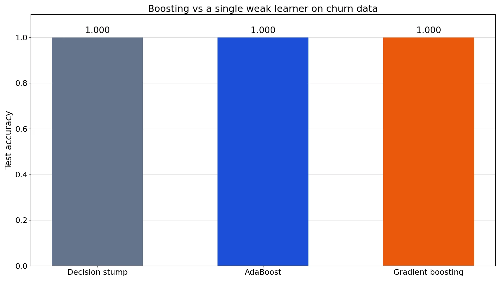
stump=1.0000, adaboost=1.0000, gradient_boosting=1.0000

The bar chart of test accuracy shows decision stump 1.000, AdaBoost 1.000, and gradient boosting 1.000.

This example is deliberately simple, and that is the point. A single stump already separates the two classes perfectly because the data is linearly separable on tenure. Boosting cannot improve on a perfect score, so both ensembles tie the stump at 1.0000 and the measured gain is 0.0000. On messy real data with overlapping classes, the same code typically shows the stump well below the ensembles. If you want the vocabulary for comparing these results with simpler reporting, see what analytics means.

How to Interpret It

Read the test accuracy as the share of held-out rows the model labels correctly. In this run, all three models score 1.0000 on 15 test rows, which means 15 correct predictions out of 15.

The more useful reading is the comparison. When the weak learner already solves the problem, the ensemble adds cost without adding accuracy. That is a signal to check whether your task is too easy, your features leak the label, or your test set is too small to distinguish models. Fifteen rows is a thin basis for any conclusion.

When the weak learner is genuinely weak, the gap between the stump and the ensemble is the value boosting adds. Track that gap, not the raw accuracy, because the gap tells you whether the sequential correction is doing work.

When to Use It (and when not to)

Use boosting when you have tabular data, a moderate number of rows, and a prediction task where a single shallow tree underfits. Gradient boosted trees are a standard choice for learning to rank, the branch of machine learning used to order results in web search engines [2]. They also handle mixed feature types and missing values well in modern implementations.

Use it when you can afford to tune. The number of iterations and the learning rate interact, and a stopping criterion such as a maximum number of iterations or a check for overfitting on a validation set is part of the workflow [1].

Do not reach for boosting when you need a model you can explain in one sentence to a non-technical audience. A single decision tree is easier to read. Do not use it when your dataset is tiny, because sequential fitting on few rows overfits quickly. Do not use it when training speed matters more than accuracy and a linear model already meets your target.

Boosting vs Bagging

Bagging and boosting are both ensembles, but they differ in how the members are built and combined.

Aspect	Boosting	Bagging
Training order	Sequential, each learner depends on the last	Parallel, learners are independent
Focus	Corrects the errors of the current model [1]	Reduces variance by averaging diverse models
Weak learner	Often a shallow tree or stump	Often a full-depth tree
Main risk	Overfitting if run too long	Underfitting if trees are too shallow
Typical examples	AdaBoost, Gradient Boosting, LogitBoost [2]	Random forests

Stochastic gradient boosting sits between the two. It subsamples the training data for each weak learner, which combines the benefits of bagging and boosting, and one variant subsamples half the data points without replacement to speed up training [2].

Common Mistakes

Assuming boosting always beats a single tree. In the worked example both ensembles tied the stump at 1.0000. Fix: always report the weak learner's score alongside the ensemble's so the gain is visible.
Setting the learning rate too high. A large shrinkage value makes each tree move the prediction a lot, which can overshoot. Fix: use a smaller learning rate and more iterations, then compare on a validation set [1].
Running too many iterations with no stopping rule. Training error can keep falling while test error rises. Fix: stop on a maximum iteration count or on validation performance [1].
Using a deep tree as the weak learner. Boosting assumes the learner is weak. Fix: keep trees shallow, often depth 1 to 3, and let the number of stages supply the capacity.
Treating the signed error as the gradient for every loss. That equivalence holds for squared error but not for other problem types [3]. Fix: specify the loss you actually care about and let the implementation compute its gradient.
Judging on a tiny test set. Fifteen rows cannot separate models that differ by a few percentage points. Fix: use a larger holdout or cross-validation.

Limitations

Boosting cannot create information that is not in your features. If the signal is absent, more stages will fit noise. The method also gives you no guarantee about the shape of the decision boundary, so a boosted model can be hard to audit even when it is accurate.

Some practitioners do not consider gradient boosting part of the boosting family at all, because it has no guarantee that training error decreases exponentially. Those algorithms are often called stagewise regression instead [2]. That naming dispute matters when you read papers, because "boosting" in one article may mean AdaBoost specifically and in another may mean the whole additive family.

Frequently Asked Questions

What is boosting in simple terms?

Boosting is a way to build one accurate model out of many weak ones. You train a simple model, find its mistakes, train the next model to fix those mistakes, and keep going. The final answer is a weighted combination of every model you trained [1].

What is the difference between AdaBoost and gradient boosting?

AdaBoost reweights the training rows so later learners focus on misclassified cases, and each learner gets a weight from its error rate [2]. Gradient boosting instead fits each new learner to the gradient of the loss function, which generalizes the idea to many loss functions beyond classification error [3].

Does boosting always improve accuracy?

No. If the weak learner already fits the data well, boosting has nothing left to correct. In the churn example, a single stump reached 1.0000 test accuracy and both ensembles matched it exactly, so the gain was 0.0000.

What does the learning rate do in boosting?

The learning rate, also called shrinkage, scales how much each weak learner contributes to the strong model [1]. A smaller value means each learner moves the prediction less, so you usually need more learners to reach the same fit.

Can boosting overfit?

Yes. Because each stage keeps reducing training error, running many iterations can fit noise. The standard control is to stop on a maximum number of iterations or when validation performance stops improving [1].