Uniform Distribution: Definition, Formula and Examples

By Dr. Zubair Khalid, DVM, MS, PhD · 2026-10-03

A uniform distribution describes a continuous variable whose values are equally likely anywhere inside a fixed interval. If you know the smallest value $a$ and the largest value $b$, you can write the density, the mean, the variance and any probability in one or two lines. This article covers the definition, the formulas, and a full worked example.

Quick Answer

A continuous uniform distribution gives equal probability density to every value between a lower bound $a$ and an upper bound $b$ [1].
The probability density function is $f(x) = \frac{1}{b - a}$ for $a \le x \le b$, and zero outside that range [1].
The mean is $\frac{a + b}{2}$ and the variance is $\frac{(b - a)^2}{12}$.
Probabilities come from the area under the flat density, so $P(X < x) = \frac{x - a}{b - a}$ for $x$ inside the interval.
The standard uniform distribution is the special case $a = 0$, $b = 1$, and it is the basis for most random number generators [1].

What Uniform Distribution Means

In plain terms, a uniform distribution is the "flat" distribution. Pick any two sub-intervals of the same width inside the range, and the variable is just as likely to fall in one as in the other. There is no peak, no tail, no center of gravity pulling values toward the middle.

The precise statistical definition: a continuous random variable $X$ follows a uniform distribution on the interval $[a, b]$ if its probability density function is constant on that interval and zero everywhere else. Because probabilities for continuous variables are measured over intervals and not at single points [2], the height of the density is not itself a probability. It is the area under the density between two points that gives the probability for that interval [2].

The uniform distribution is one of the core continuous probability models, alongside the normal and exponential families. If you are new to the general idea, start with probability distributions explained and then come back here.

How It Works

The probability density function (PDF) of a continuous uniform variable is:

$$f(x) = \frac{1}{b - a} \quad \text{for } a \le x \le b$$

Each symbol means the following.

$x$ is the value of the random variable.
$a$ is the lower bound of the interval, sometimes called the location parameter [1].
$b$ is the upper bound.
$b - a$ is the width of the interval, sometimes called the scale parameter [1].

Outside the interval $[a, b]$, the density is zero. The density is flat, so the total area under it is a rectangle of height $\frac{1}{b - a}$ and width $b - a$, which equals 1, as any density must [2].

The cumulative distribution function (CDF) gives the probability that $X$ is at most some value $x$:

$$F(x) = P(X \le x) = \frac{x - a}{b - a} \quad \text{for } a \le x \le b$$

The mean and variance are:

$$\mu = \frac{a + b}{2} \qquad \sigma^2 = \frac{(b - a)^2}{12}$$

The mean is simply the midpoint of the interval. The variance grows with the square of the width, so doubling the range quadruples the variance. The standard deviation is the square root of the variance.

For the standard uniform distribution with $a = 0$ and $b = 1$, the density is $f(x) = 1$ on the interval and the CDF is $F(x) = x$ [1]. Most random number generators produce values on the $(0, 1)$ interval, and other distributions are obtained by transforming those values [1].

Worked Example

Suppose a city bus arrives on a fixed schedule, and you walk up to the stop at a random moment. Your wait time in minutes is modeled as $X \sim \text{Uniform}(a = 0, b = 15)$. Twelve recorded wait times from that stop are shown below.

wait_minutes
1.2
3.4
5.1
6.8
8.3
9.9
11.2
12.6
13.8
14.5
2.7
7.4

Step 1. State the distribution. The wait is uniform from 0 to 15 minutes, so $X \sim \text{Uniform}(a = 0, b = 15)$.

Step 2. Write the PDF. The density is constant across the interval:

$$f(x) = \frac{1}{b - a} = \frac{1}{15 - 0} = 0.0667$$

Step 3. Compute the mean. The expected wait is the midpoint:

$$\mu = \frac{a + b}{2} = \frac{0 + 15}{2} = 7.5000$$

Step 4. Compute the variance and standard deviation:

$$\sigma^2 = \frac{(b - a)^2}{12} = \frac{(15 - 0)^2}{12} = 18.7500$$

$$\sigma = \sqrt{18.7500} = 4.3301$$

Step 5. Compute a probability. The chance of waiting less than 5 minutes is the area under the density from 0 to 5:

$$P(X < 5) = \frac{x - a}{b - a} = \frac{5 - 0}{15 - 0} = 0.3333$$

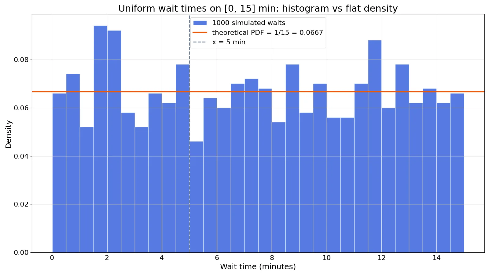
Step 6. Check with a simulation. Drawing 1000 values from this distribution gives a simulated mean of 7.4577 and a simulated fraction under 5 minutes of 0.3460. Both sit close to the theoretical values of 7.5000 and 0.3333, which is what you expect from random sampling.

The same numbers come out of a few lines of Python using SciPy's uniform object, which is parameterized by loc (the lower bound) and scale (the width $b - a$) [3].

from scipy.stats import uniform
a, b, x = 0, 15, 5
d = uniform(loc=a, scale=b-a)
print(f"pdf(7) = {d.pdf(7):.4f}, mean = {d.mean():.4f}, var = {d.var():.4f}, P(X<5) = {d.cdf(x):.4f}")

Output:

pdf(7) = 0.0667, mean = 7.5000, var = 18.7500, P(X<5) = 0.3333

How to Interpret It

The density value 0.0667 is not a probability. It is the height of a flat line, and only areas under that line are probabilities [2]. The rectangle from 0 to 5 has width 5 and height 0.0667, so its area is 0.3333, which matches the CDF calculation.

The mean of 7.5 minutes is the balance point of the interval, not a value you expect to see more often than any other. Every wait time between 0 and 15 minutes has the same density. The standard deviation of 4.3301 minutes tells you how spread out the waits are around that midpoint.

Because the density is flat, the median and the mean are the same value, and the distribution is symmetric. That symmetry is a useful check when you fit a uniform model to data. If your histogram is visibly skewed, a uniform model is the wrong choice. For skewed data, compare with the exponential distribution or read about a right skewed distribution.

When to Use It (and when not to)

Use a uniform distribution when the interval is known and every value inside it is equally plausible. Common cases include random number generation on $(0, 1)$ [1], rounding errors within a fixed precision, and arrival times when you know only that an event is equally likely at any moment in a window.

Use it when you have only the minimum and maximum of a range and no reason to expect a peak. The statistical range gives you $b - a$ directly, which is all the uniform model needs.

Do not use it when the data cluster near a center. Real wait times, heights, measurement errors and test scores usually peak somewhere, and a normal or exponential model fits better. Do not use it for counts or other discrete outcomes. Those need a discrete model such as the binomial distribution or the Poisson distribution. You can test discrete counts quickly with a binomial distribution calculator.

Uniform Distribution vs Normal Distribution

The closest related idea is the normal distribution, which also describes continuous variables on a range. The difference is the shape.

Feature	Uniform	Normal
Shape	Flat rectangle	Bell curve
Parameters	$a$ and $b$	Mean $\mu$ and standard deviation $\sigma$
Mean	$(a + b)/2$	$\mu$
Variance	$(b - a)^2/12$	$\sigma^2$
Range	Bounded, $[a, b]$	Unbounded in theory
Typical use	Random draws, unknown position in a window	Measurements that cluster near a center

If your histogram looks like a rectangle, use the uniform model. If it looks like a hill, use the normal distribution. For a deeper look at the density concept itself, see probability density function.

Common Mistakes

Treating the density height as a probability. The value $0.0667$ is a density, not a chance. Fix: always compute an area, using $P(X < x) = \frac{x - a}{b - a}$.
Forgetting that $P(X = x) = 0$ for any single point. For continuous variables, probabilities are measured over intervals, not single points [2]. Fix: ask for a range, not an exact value.
Mixing up $b$ and the width. The density uses $b - a$, not $b$. Fix: compute the width first and label it clearly.
Using the uniform model on peaked data. A flat model on a bell-shaped histogram gives badly wrong tail probabilities. Fix: plot the data before choosing a model.
Assuming the interval bounds are exact. If $a$ and $b$ are estimated from a small sample, the probabilities inherit that uncertainty. Fix: report the bounds and the sample size together.
Confusing the discrete and continuous versions. A discrete uniform variable has a finite list of equally likely values, and its probabilities are sums, not areas. Fix: check whether the variable is a count or a measurement.

Limitations

The uniform distribution cannot describe data that cluster, taper or have outliers. It forces a flat shape on everything, so if the true process peaks in the middle, the model will underestimate central probabilities and overestimate tail probabilities. It also assumes hard boundaries. Real measurements often have soft edges, where the density fades instead of stopping abruptly.

The model is only as good as the bounds you supply. If $a$ and $b$ come from a small sample, they are estimates, and the resulting mean, variance and probabilities carry that sampling error. The uniform distribution also says nothing about dependence between observations. If your wait times are correlated across days, a single uniform model will understate the real variability.

Frequently Asked Questions

What is the formula for the uniform distribution?

The probability density function is $f(x) = \frac{1}{b - a}$ for $a \le x \le b$, and zero outside that interval [1]. The cumulative distribution function is $F(x) = \frac{x - a}{b - a}$ inside the interval. The mean is $\frac{a + b}{2}$ and the variance is $\frac{(b - a)^2}{12}$.

What is the difference between a discrete and a continuous uniform distribution?

A discrete uniform distribution assigns equal probability to a finite set of values, such as the outcomes of a fair die. A continuous uniform distribution assigns equal probability density to every point in an interval, so probabilities come from areas rather than sums [2]. The continuous version is the one used for random number generation on $(0, 1)$ [1].

How do you calculate the probability between two values?

Subtract the lower bound from the upper value of interest, then divide by the width of the interval. For $X \sim \text{Uniform}(0, 15)$, the probability of a wait under 5 minutes is $\frac{5 - 0}{15 - 0} = 0.3333$. The same logic works for any sub-interval inside $[a, b]$.

What are the mean and variance of a uniform distribution?

The mean is the midpoint, $\frac{a + b}{2}$. The variance is $\frac{(b - a)^2}{12}$, and the standard deviation is its square root. For $a = 0$ and $b = 15$, the mean is 7.5000, the variance is 18.7500 and the standard deviation is 4.3301.

Can the uniform distribution have a density greater than 1?

Yes. The density must integrate to 1 over the interval, but its height can exceed 1 when the interval is narrow [2]. For example, a uniform distribution on $[0, 0.5]$ has density 2. Only the area under the density is a probability, and that area is always between 0 and 1.