Normal PDF: Formula, Definition and Examples
By Dr. Zubair Khalid, DVM, MS, PhD ·
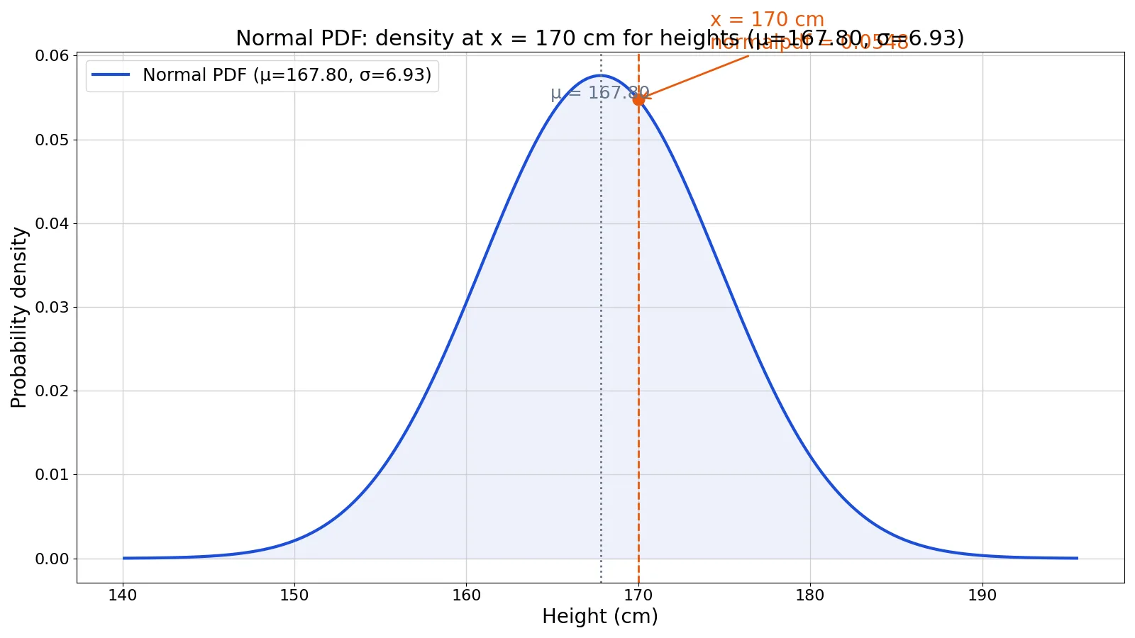
The normalpdf is the probability density function (PDF) of the normal distribution. It returns the height of the bell curve at a given value $x$, not the probability of landing exactly on $x$. You use it to draw the curve, compare how likely different values are, and build the probabilities that the normal CDF reports.
Quick Answer
- The normalpdf formula is $f(x) = \dfrac{1}{\sigma\sqrt{2\pi}}\, e^{-\frac{(x-\mu)^2}{2\sigma^2}}$, where $\mu$ is the mean and $\sigma$ is the standard deviation.
- It takes three inputs: the value $x$, the mean $\mu$, and the standard deviation $\sigma$.
- The output is a density, so it can be greater than 1 when $\sigma$ is small. It is not a probability.
- Probabilities come from the area under the curve, which you get from the normal CDF or by integrating the PDF.
- In Python,
scipy.stats.norm.pdf(x, loc=mu, scale=sd)returns the same value as the formula.
Syntax
The function appears in different tools under slightly different names, but the arguments are the same idea. The table below describes the general argument set.
| Argument | Required? | Meaning |
|---|---|---|
| x | Yes | The value at which you evaluate the density. Any real number. |
| mean (μ) | Yes | The center of the distribution. |
| standard_deviation (σ) | Yes | The spread of the distribution. Must be greater than 0. |
| cumulative | Yes in Excel | A flag in some tools. When false, you get the PDF. When true, you get the CDF. |
In Excel, the function is NORM.DIST, and the fourth argument cumulative decides between PDF and CDF. In Python, norm.pdf and norm.cdf are separate functions. The NORM.DIST formula in Excel covers the spreadsheet version in detail.
How It Works
The formula has two parts that multiply together.
$$f(x) = \underbrace{\frac{1}{\sigma\sqrt{2\pi}}}_{\text{constant}} \times \underbrace{e^{-\frac{(x-\mu)^2}{2\sigma^2}}}_{\text{exponential term}}$$
The constant $1/(\sigma\sqrt{2\pi})$ scales the curve so the total area under it equals 1. A larger $\sigma$ makes this constant smaller, which flattens and widens the curve. A smaller $\sigma$ makes it larger, which produces a tall, narrow peak.
The exponential term measures how far $x$ sits from the mean in standard deviation units. Define the z-score as $z = (x-\mu)/\sigma$. Then the exponential term becomes $e^{-z^2/2}$. At $x = \mu$, the z-score is 0 and the term equals 1, so the density peaks there. As $x$ moves away from the mean, the term shrinks toward 0.
This is why the density is highest at the mean and never quite reaches zero in the tails. The curve is symmetric around $\mu$, so $f(\mu - d) = f(\mu + d)$ for any distance $d$.
Changing $\mu$ slides the curve left or right without changing its shape. Changing $\sigma$ changes the shape. The normal distribution article shows both effects with animated plots.
One point trips people up. The density value is not a probability. For a continuous variable, the probability of any single exact value is zero. Density only becomes probability when you multiply it by a width or integrate it over an interval. That distinction is the core of the difference between CDF and PDF.
Worked Example
The dataset is the height in centimeters of 30 students in a class. We want the normalpdf at $x = 170$ cm using the sample mean and sample standard deviation.
| student_id | height_cm | student_id | height_cm | student_id | height_cm |
|---|---|---|---|---|---|
| 1 | 152 | 11 | 166 | 21 | 170 |
| 2 | 155 | 12 | 166 | 22 | 171 |
| 3 | 158 | 13 | 167 | 23 | 172 |
| 4 | 160 | 14 | 167 | 24 | 173 |
| 5 | 161 | 15 | 168 | 25 | 174 |
| 6 | 162 | 16 | 168 | 26 | 175 |
| 7 | 163 | 17 | 168 | 27 | 176 |
| 8 | 164 | 18 | 169 | 28 | 178 |
| 9 | 165 | 19 | 169 | 29 | 180 |
| 10 | 165 | 20 | 170 | 30 | 182 |
Step 1. Sample size.
$$n = 30$$
Step 2. Sample mean. The heights sum to 5034.
$$\mu = \frac{\sum x}{n} = \frac{5034}{30} = 167.8000$$
Step 3. Sample standard deviation, using $n-1$ in the denominator.
$$\sigma = 6.9252$$
Step 4. Standardize $x = 170$.
$$z = \frac{170 - 167.8000}{6.9252} = 0.3177$$
Step 5. Compute the normalization constant. Note that $\sqrt{2\pi} \approx 2.5066$.
$$\frac{1}{\sigma\sqrt{2\pi}} = \frac{1}{6.9252 \times 2.5066} = 0.0576$$
Step 6. Compute the exponential term.
$$e^{-z^2/2} = e^{-0.3177^2/2} = 0.9508$$
Step 7. Multiply the two parts.
$$f(170) = 0.0576 \times 0.9508 = 0.0548$$
So the normalpdf at 170 cm is 0.0548. A value close to the mean gives a density near the peak. Since 170 is only about a third of a standard deviation above the mean, the density is still high.
Here is the same calculation in Python.
from scipy.stats import norm
import numpy as np
heights = [152, 155, 158, 160, 161, 162, 163, 164, 165, 165,
           166, 166, 167, 167, 168, 168, 168, 169, 169, 170,
           170, 171, 172, 173, 174, 175, 176, 178, 180, 182]
mu = np.mean(heights)   # 167.8000
sd = np.std(heights, ddof=1)  # 6.9252
print(f"mean = {mu:.4f}")
print(f"sd   = {sd:.4f}")
print(f"normalpdf(170) = {norm.pdf(170, loc=mu, scale=sd):.4f}")
Output:
mean = 167.8000
sd   = 6.9252
normalpdf(170) = 0.0548
The density curve for these heights has its peak at 167.80 cm and a spread of 6.93 cm. The point $x = 170$ cm sits just right of center with a density of 0.0548.
More Examples
Density at the mean. Set $x = \mu = 167.8000$. Then $z = 0$ and the exponential term is 1, so the density is just the constant, 0.0576. That is the peak height of this curve.
Density far in the tail. Set $x = 182$, the tallest student. The z-score is $(182 - 167.8000)/6.9252 = 2.0505$. The exponential term is $e^{-2.0505^2/2} = 0.1222$, and the density is $0.0576 \times 0.1222 = 0.0070$. The curve is much lower out there.
Standard normal case. With $\mu = 0$ and $\sigma = 1$, the constant is $1/\sqrt{2\pi} = 0.3989$. At $x = 0$ the density is 0.3989. At $x = 1$ it is $0.3989 \times e^{-0.5} = 0.2420$. These are the values behind the standard normal table.
Turning density into probability. To get the probability that a student is between 165 cm and 170 cm, you integrate the PDF over that range, or subtract two CDF values. The density alone does not answer that question.
Errors and How to Fix Them
Negative or zero standard deviation. The formula divides by $\sigma$, so $\sigma = 0$ is undefined and negative values are invalid. Check that your spread measure is positive. If your data are all identical, the normal model does not apply.
Passing variance where standard deviation belongs. Some tools name the argument scale and expect $\sigma$, while others ask for variance $\sigma^2$. In Python, norm.pdf(x, loc=mu, scale=sd) wants the standard deviation. Passing 47.96 (the variance of this dataset) instead of 6.9252 gives a density of 0.0083, which is wrong.
Forgetting the cumulative flag in Excel. NORM.DIST(x, mean, sd, FALSE) returns the PDF. If you set it to TRUE, you get the CDF instead (0.6246 at 170 cm in the height example). If you leave the flag out, Excel rejects the formula because the argument is required.
Reading the output as a probability. A density of 0.0548 does not mean a 5.48% chance that a student is exactly 170 cm tall. That probability is zero for a continuous variable.
Mixing units. If $x$ is in centimeters, $\mu$ and $\sigma$ must also be in centimeters. A mismatch silently produces a meaningless number.
Common Mistakes
- Treating the density as a probability. Fix: integrate over an interval or use the CDF for any probability question.
- Using the population standard deviation when you have a sample and want the sample spread. Fix: use $n-1$ in the denominator, as in the worked example.
- Assuming the density must be below 1. Fix: remember that density is scaled by $1/\sigma$, so small spreads give tall curves with values above 1.
- Plugging in the variance instead of the standard deviation. Fix: take the square root first, then pass that value.
- Comparing densities across variables with different units. Fix: standardize to z-scores before comparing.
- Expecting the normalpdf to tell you how well data fit a normal curve. Fix: use a histogram, a Q-Q plot, or a formal normality test.
Limitations
The normalpdf describes a theoretical curve, not your data. It assumes the variable is continuous, symmetric, and fully described by its mean and standard deviation. Real data with skew, outliers, or hard boundaries will not match the curve well, and the density values will mislead you about how common extreme values are.
The density is also not a probability, so it cannot answer "what is the chance of exactly this value" for a continuous variable. And the formula says nothing about whether the normal model is appropriate in the first place. That judgment comes from the data, not from the function.
Frequently Asked Questions
What is the difference between normalpdf and normalcdf?
The normalpdf gives the height of the density curve at a single point. The normalcdf gives the area under the curve up to a point, which is a probability. Use the PDF to draw the curve or compare relative likelihoods. Use the CDF to answer questions like "what fraction of students are under 170 cm."
Can normalpdf return a value greater than 1?
Yes. The density is scaled by $1/(\sigma\sqrt{2\pi})$, so when $\sigma$ is small the peak can exceed 1. For example, with $\sigma = 0.1$ the peak density is about 3.99. This is fine because density is not a probability.
What happens if I use the wrong standard deviation?
The curve changes shape and every density value shifts. In the height example, using the variance 47.96 instead of the standard deviation 6.9252 gives 0.0083 at $x = 170$ instead of 0.0548. Always confirm whether your tool wants $\sigma$ or $\sigma^2$.
How do I compute normalpdf in Excel?
Use NORM.DIST(x, mean, standard_deviation, FALSE). The FALSE flag selects the PDF. Setting it to TRUE returns the CDF. For the height example, NORM.DIST(170, 167.8, 6.9252, FALSE) returns 0.0548.
Why is the density at the mean the highest point?
At $x = \mu$ the z-score is 0, so the exponential term $e^{-z^2/2}$ equals 1, its maximum. Every other value of $x$ makes the exponent negative and shrinks the term. That is why the peak sits at the mean and the curve falls away on both sides.
References
This article draws on the standard references listed under Further Reading.
Further Reading
- normal.html
- normal.html
- Altman DG, Bland JM (1995). Statistics notes: The normal distribution. BMJ
- NIST/SEMATECH e-Handbook of Statistical Methods
- OpenStax. Introductory Statistics 2e
- Krzywinski M, Altman N (2013). Importance of being uncertain. Nature Methods