Excel SUMPRODUCT Function: Syntax and Examples

By Dr. Zubair Khalid, DVM, MS, PhD · 2026-10-03

Excel SUMPRODUCT multiplies corresponding values in two or more arrays and returns the sum of those products. It is the standard way to compute a sum of products in one formula, and it also handles conditional totals without helper columns. This article covers the syntax, how the calculation runs, and worked examples you can copy.

Quick Answer

SUMPRODUCT takes two or more arrays of equal size, multiplies the values position by position, and adds the results.
The basic form is =SUMPRODUCT(array1, array2). With quantities in one column and prices in another, it returns total revenue in a single cell.
Arrays must have the same dimensions. A mismatch returns the #VALUE! error.
Conditions work by multiplying arrays of TRUE and FALSE values into the calculation, so only matching rows contribute.
Text and logical values inside the arrays are treated as zero, which is why SUMPRODUCT tolerates labels and blanks better than arithmetic on whole columns.

Syntax

=SUMPRODUCT(array1, [array2], [array3], ...)

Argument	Required?	Meaning
array1	Required	The first array or range. Its values are multiplied by the matching values in the other arrays.
array2	Optional	The second array or range. Must have the same number of rows and columns as array1.
array3, ...	Optional	Further arrays, each matching the dimensions of array1. Excel accepts up to 255 arguments.

If you supply only one array, SUMPRODUCT simply adds its values, which makes it behave like a SUM formula for that range. With two or more arrays, it performs the multiply-then-add operation.

How It Works

SUMPRODUCT walks through the arrays in parallel. For each position, it takes the value from array1, the value from array2, and so on, multiplies them together, and keeps a running total. When it reaches the end, it returns that total.

For two arrays of length $n$, the result is:

$$\text{SUMPRODUCT}(A,B) = \sum_{i=1}^{n} A_i \times B_i$$

This is the same arithmetic you would get from a helper column of =A2*B2 formulas followed by a SUM, but it happens inside one cell. That matters when you want a clean sheet or when the intermediate products have no meaning on their own.

The conditional behavior comes from the same arithmetic. A comparison such as A2:A6="Widget" returns an array of TRUE and FALSE values. When you multiply that array by numeric arrays, TRUE acts as 1 and FALSE acts as 0, so non-matching rows contribute nothing to the total. This is the mechanism behind conditional sums, and it is why SUMPRODUCT can replace a SUMIF or SUMIFS formula in many cases.

One practical detail: SUMPRODUCT does not need to be entered as an array formula in modern Excel. You type it normally and press Enter.

Worked Example

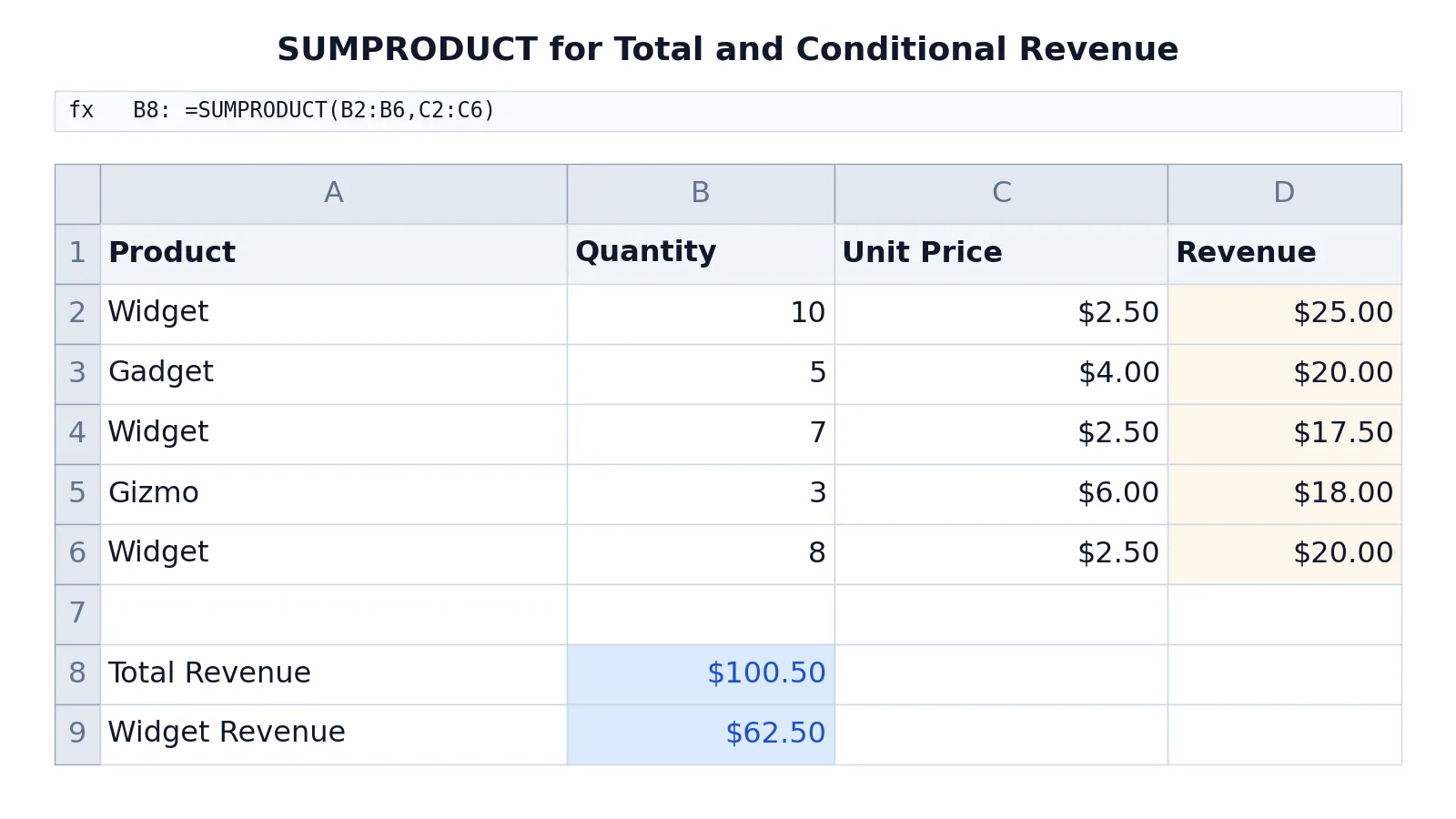
The table below tracks product sales, with quantity and unit price for each row. Column D shows the per-row revenue that SUMPRODUCT replaces.

	A	B	C	D
1	Product	Quantity	Unit Price	Revenue
2	Widget	10	2.5	`=B2*C2 -> displays $25.00`
3	Gadget	5	4	`=B3*C3 -> displays $20.00`
4	Widget	7	2.5	`=B4*C4 -> displays $17.50`
5	Gizmo	3	6	`=B5*C5 -> displays $18.00`
6	Widget	8	2.5	`=B6*C6 -> displays $20.00`
8	Total Revenue	`=SUMPRODUCT(B2:B6,C2:C6) -> displays $100.50`
9	Widget Revenue	`=SUMPRODUCT((A2:A6="Widget")B2:B6C2:C6) -> displays $62.50`

Cell B8 multiplies each quantity by its unit price and sums the results to get total revenue. The five products are 25.00, 20.00, 17.50, 18.00 and 20.00, which add to 100.50.

Cell B9 multiplies quantity by unit price only for rows where the product is Widget, then sums those revenues. The Widget rows are 2, 4 and 6, giving 25.00, 17.50 and 20.00, which add to 62.50.

The condition sits inside the formula as (A2:A6="Widget"). The parentheses matter. Without them, Excel would evaluate the comparison against the wrong part of the expression.

More Examples

Weighted average. If scores are in B2:B10 and weights in C2:C10, the weighted average is =SUMPRODUCT(B2:B10,C2:C10)/SUM(C2:C10). The numerator is the sum of products, and the denominator normalizes by total weight.

Count with two conditions. SUMPRODUCT can count rows that meet several criteria. =SUMPRODUCT((A2:A100="Widget")*(B2:B100>5)) returns the number of Widget rows with quantity above 5. Each condition produces a 0 or 1 array, and the product is 1 only when both are true. For simple counting tasks, a COUNT formula is often easier, but SUMPRODUCT handles multiple conditions without extra arguments.

Sum with OR logic. To total revenue for Widgets or Gizmos, add the condition arrays instead of multiplying them: =SUMPRODUCT(((A2:A6="Widget")+(A2:A6="Gizmo"))*B2:B6*C2:C6). The plus sign acts as OR, and any row matching either product contributes.

Sum with a numeric condition. =SUMPRODUCT((C2:C6>3)*B2:B6*C2:C6) totals revenue only for rows where the unit price exceeds 3. This pattern extends to any number of conditions by multiplying more arrays together.

Using SUMPRODUCT with other functions. You can nest results from other formulas inside the arrays. For example, if you build labels with a TEXT formula or extract characters with a RIGHT formula, those outputs can feed a SUMPRODUCT condition as long as the arrays line up.

Errors and How to Fix Them

#VALUE! from mismatched dimensions. SUMPRODUCT requires every array to have the same number of rows and columns. If one range is B2:B6 and another is C2:C7, the formula fails. Fix it by aligning the ranges exactly.

#VALUE! from text in a numeric array. When you multiply arrays with * inside the formula, text that cannot be coerced to a number makes the multiplication fail. The comma-separated form treats that text as zero instead. Check for stray labels or notes typed into the quantity or price columns.

Wrong totals from whole-column references. =SUMPRODUCT(B:B,C:C) includes the header row and any text below the data. Headers are text, so they are treated as zero, but stray numbers far down the column will be counted. Use bounded ranges such as B2:B1000.

Conditions returning everything or nothing. A condition like (A2:A6="widget") is case-insensitive in Excel, so it matches "Widget" and "WIDGET". If your total looks wrong, check the comparison text and the parentheses around the condition.

Unexpected results from blanks. Empty cells are treated as zero in the multiplication, which is usually what you want. If a blank should be excluded rather than counted as zero, add a condition that tests for non-blank cells.

Common Mistakes

Forgetting parentheses around conditions. A2:A6="Widget"*B2:B6 is not the same as (A2:A6="Widget")*B2:B6. The first version compares a text value to a number and returns an error. Wrap each condition in parentheses.
Mixing OR and AND logic. Multiplying condition arrays means AND, adding them means OR. Using the wrong operator silently returns a plausible but incorrect total. Decide which logic you need before writing the formula.
Using mismatched range sizes. A condition on A2:A6 combined with B2:B10 breaks the calculation. Keep every range the same height and width.
Assuming SUMPRODUCT is always faster than SUMIFS. For large datasets, SUMIFS is often more efficient because it is optimized for criteria-based aggregation. SUMPRODUCT is more flexible, not automatically quicker.
Leaving helper-column arithmetic in place. If you already have a revenue column, =SUM(D2:D6) is simpler and easier to audit. Use SUMPRODUCT when you want to avoid the helper column or need array logic.
Ignoring the single-array case. =SUMPRODUCT(B2:B6) just adds the quantities. If you expected a product, you forgot the second array.

Limitations

SUMPRODUCT cannot return more than one value. It always collapses to a single number, so it is not a replacement for dynamic array functions when you need a spilled result. It also cannot handle arrays of different shapes, which rules out some cross-table calculations that a lookup function would handle.

Performance is the other constraint. Every array in the formula is evaluated element by element, so a SUMPRODUCT over hundreds of thousands of rows with several conditions can slow a workbook noticeably. For repeated aggregation on large tables, a PivotTable or a dedicated aggregation function is usually the better tool. SUMPRODUCT also treats text as zero without warning, so a mislabeled column can produce a total that looks reasonable but is missing data.

Frequently Asked Questions

What is the difference between SUMPRODUCT and SUM?

SUM adds the values in a range. SUMPRODUCT multiplies matching values across two or more ranges first, then adds the products. If you need a plain total, use SUM. If you need quantity times price, use SUMPRODUCT.

Can SUMPRODUCT handle multiple conditions?

Yes. Multiply condition arrays together for AND logic, or add them for OR logic, then multiply by the value arrays. Each condition returns TRUE or FALSE, which behaves as 1 or 0 in the arithmetic.

Why does my SUMPRODUCT return #VALUE!?

The most common cause is arrays with different dimensions. Check that every range has the same number of rows and columns. Text inside a numeric array can also trigger the error.

Is SUMPRODUCT case-sensitive?

No. Text comparisons inside SUMPRODUCT are case-insensitive, so "Widget" and "widget" match the same rows. If you need a case-sensitive match, use an exact comparison function inside the condition.

Does SUMPRODUCT work with dates?

Yes. Dates are stored as serial numbers, so comparisons such as (A2:A100>=DATE(2024,1,1)) work normally. The result is a count or sum of the rows that fall in the date range you specify.

References

This article draws on the standard references listed under Further Reading.