How to Use the IF Function in Excel (Step by Step)
By Dr. Zubair Khalid, DVM, MS, PhD ·
The if formula in Excel tests a condition and returns one value when the test is true and a different value when it is false. You write it as =IF(logical_test, value_if_true, value_if_false), so a formula like =IF(B2>=70,"Pass","Fail") labels a score as Pass or Fail in a single step [1]. This guide covers the syntax, a worked example on real student data, nested IF, and IF combined with AND and OR.
Quick Answer
- The IF function has three arguments: the test, the value to return when the test is true, and the value to return when it is false [1].
- The third argument is optional in the syntax, but leaving it out returns FALSE when the test fails, so most formulas supply it [1].
- IF can compare text as well as numbers, for example
=IF(C2="Yes",1,2)[1]. - To test more than one condition, put AND or OR inside the test, as in
=IF(AND(B2>=70,D2>=0.8),"Pass","Fail")[2]. - Nest IF inside IF to handle several ranges, but keep the nesting shallow and consider the IFS function instead [3].
Syntax
| Argument | Required? | Meaning |
|---|---|---|
| logical_test | Required | The condition you want to check. It must evaluate to TRUE or FALSE [4]. |
| value_if_true | Required | The value returned if the result of logical_test is TRUE [1]. |
| value_if_false | Optional | The value returned if the result of logical_test is FALSE [1]. |
The full form is:
$$=IF(logical\_test,\ value\_if\_true,\ [value\_if\_false])$$
How It Works
Excel evaluates the logical_test first. The test is any expression that produces TRUE or FALSE, such as B2>=70, C2="Yes", or A2<>"Sprockets" [4]. If the test is TRUE, Excel returns the second argument. If it is FALSE, Excel returns the third argument [1].
Text results need double quotes around them, as in "Pass". Numbers do not. You can also return a calculation instead of a fixed value, so =IF(E2<31500,E2*15%,E2*25%) multiplies the cell by one rate or another depending on the income level [5].
When you copy a formula down a column, relative references adjust automatically. A formula written in C2 as =IF(B2>=70,"Pass","Fail") becomes =IF(B3>=70,"Pass","Fail") in C3, and so on down the column.
To test several conditions at once, use AND or OR as the logical_test. AND returns TRUE only if every argument is TRUE [6]. OR returns TRUE if any argument is TRUE [7]. Wrapping either one inside IF gives you a multi-condition rule:
$$=IF(AND(Something\ is\ True,\ Something\ else\ is\ True),\ Value\ if\ True,\ Value\ if\ False)$$
Worked Example
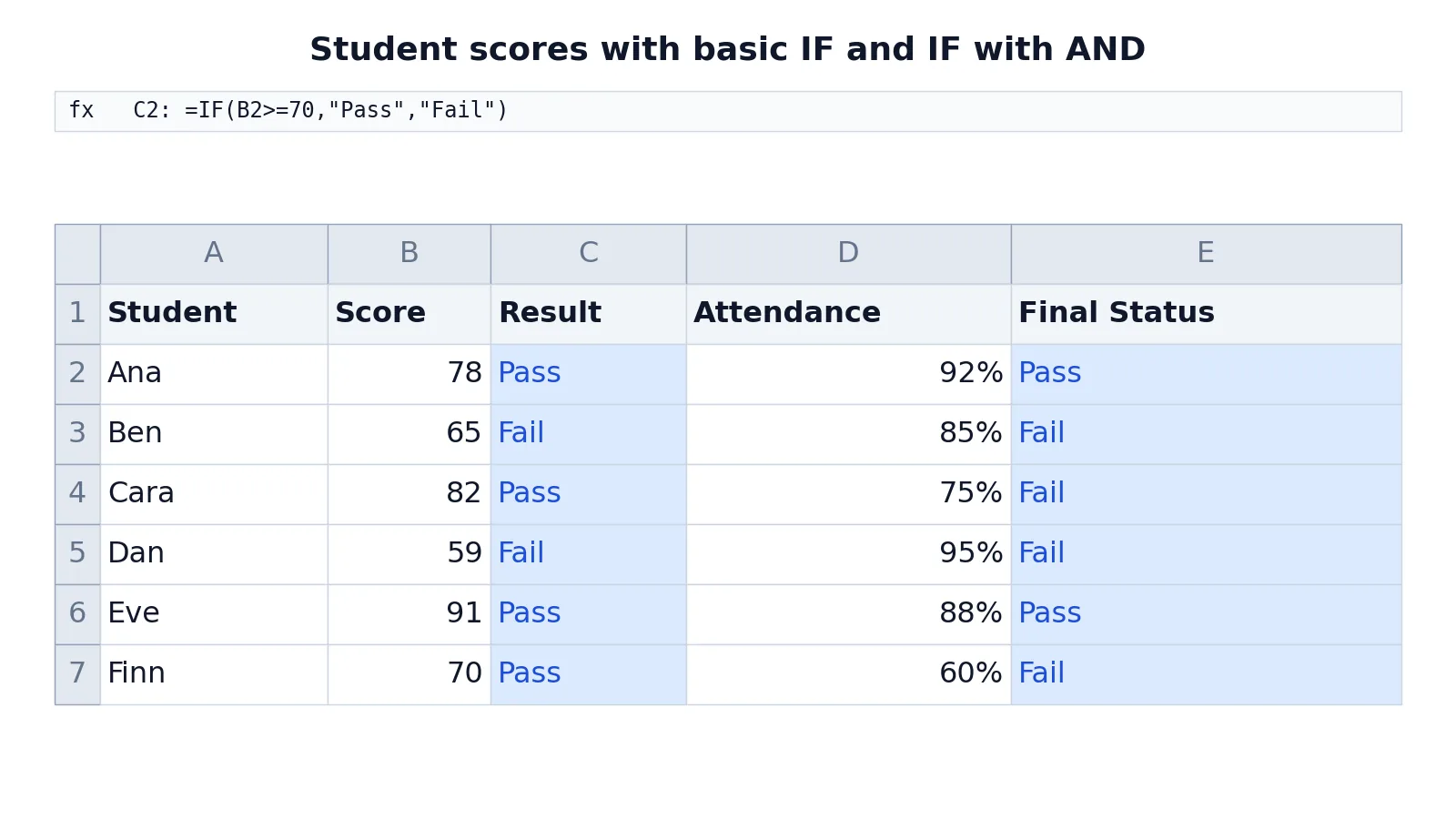
The table below tracks six students with a score, an attendance rate, a basic IF result in column C, and an IF with AND result in column E. Column C passes a student when the score is at least 70. Column E passes a student only when the score is at least 70 and attendance is at least 0.8.
| A | B | C | D | E | |
|---|---|---|---|---|---|
| 1 | Student | Score | Result | Attendance | Final Status |
| 2 | Ana | 78 | =IF(B2>=70,"Pass","Fail") -> displays Pass | 0.92 | =IF(AND(B2>=70,D2>=0.8),"Pass","Fail") -> displays Pass |
| 3 | Ben | 65 | =IF(B3>=70,"Pass","Fail") -> displays Fail | 0.85 | =IF(AND(B3>=70,D3>=0.8),"Pass","Fail") -> displays Fail |
| 4 | Cara | 82 | =IF(B4>=70,"Pass","Fail") -> displays Pass | 0.75 | =IF(AND(B4>=70,D4>=0.8),"Pass","Fail") -> displays Fail |
| 5 | Dan | 59 | =IF(B5>=70,"Pass","Fail") -> displays Fail | 0.95 | =IF(AND(B5>=70,D5>=0.8),"Pass","Fail") -> displays Fail |
| 6 | Eve | 91 | =IF(B6>=70,"Pass","Fail") -> displays Pass | 0.88 | =IF(AND(B6>=70,D6>=0.8),"Pass","Fail") -> displays Pass |
| 7 | Finn | 70 | =IF(B7>=70,"Pass","Fail") -> displays Pass | 0.6 | =IF(AND(B7>=70,D7>=0.8),"Pass","Fail") -> displays Fail |
Read the two columns together and the difference between a single test and a combined test becomes clear. Cara scores 82, so column C says Pass, but her attendance of 0.75 falls below 0.8, so column E says Fail. Finn scores exactly 70, which satisfies >=70, so column C says Pass, but his attendance of 0.6 fails the second condition and column E says Fail. Dan has strong attendance at 0.95 but a score of 59, so both columns say Fail. Only Ana and Eve clear both thresholds.
The >= operator matters here. If you wrote >70 instead, Finn would fail column C because 70 is not greater than 70. Choosing the right comparison operator is part of writing the rule correctly.
More Examples
A nested IF handles more than two outcomes. The classic grading pattern checks each threshold in turn [3]:
=IF(D2>89,"A",IF(D2>79,"B",IF(D2>69,"C",IF(D2>59,"D","F"))))Excel reads this from the outside in. If the score is above 89, the formula returns A and stops. Otherwise it moves to the next test, and so on. The same logic can be written with a single IFS function, which removes the pile of closing parentheses [3]:
=IFS(D2>89,"A",D2>79,"B",D2>69,"C",D2>59,"D",TRUE,"F")For a two-condition rule where either condition is enough, use OR. The pattern below awards a commission when total sales meet the goal or accounts meet the account goal [7]:
=IF(OR(B14>=$B$4,C14>=$B$5),B14*$B$6,0)The AND version of the same idea pays a bonus only when both targets are met [6]:
=IF(AND(B14>=$B$7,C14>=$B$5),B14*$B$8,0)If you want to return a calculation rather than a label, put the arithmetic in the value arguments. The income example below applies a 15 percent rate under 31,500, a 25 percent rate under 72,500, and 28 percent above that [5]:
=IF(E2<31500,E2*15%,IF(E2<72500,E2*25%,E2*28%))Errors and How to Fix Them
An error result is the most common IF problem. When an argument refers to a cell that already contains an error value, such as #VALUE! or #N/A, IF returns that error instead of a result [5]. Check the cells your formula points at and clear the upstream error first.
A missing quote is the next frequent cause. Text values must sit inside double quotes, so "Pass" works and Pass does not. Excel will either reject the formula or treat the bare word as a defined name.
Unbalanced parentheses produce a different message. Count the opening and closing brackets, or let Excel highlight the matching pair as you type. Deeply nested IF formulas are the usual source of this problem [3].
If you cannot avoid an error in the data, wrap the whole formula in IFERROR to substitute a fallback value [5]:
=IFERROR(IF(E2<31500,E2*15%,IF(E2<72500,E2*25%,E2*28%)),0)Common Mistakes
- Using
>when you mean>=. A threshold of 70 written as>70excludes anyone who scores exactly 70. Decide whether the boundary belongs to the pass group and pick the operator to match. - Forgetting quotes around text.
=IF(B2>=70,Pass,Fail)fails because Pass and Fail are not quoted. Write"Pass"and"Fail". - Nesting too deeply. Excel allows up to 64 nested IF functions, but that is not advisable [3]. Switch to IFS or a lookup table once you pass three or four levels.
- Leaving out the false argument. The third argument is optional, so
=IF(B2>=70,"Pass")returns FALSE for low scores instead of a label [1]. Supply the value you actually want. - Mixing AND and OR logic. AND requires every condition to be true, OR requires just one [6][7]. Pick the one that matches the business rule before you write the formula.
- Hardcoding thresholds in many formulas. If the cutoff changes, you must edit every cell. Put the threshold in its own cell and reference it.
Limitations
IF returns exactly one of two values per test, so it cannot express three or more outcomes without nesting or switching to IFS [3]. Each added layer makes the formula harder to read and easier to break, and a misplaced parenthesis can be difficult to spot in a long chain.
IF also does not handle errors in the tested cells on its own. If a referenced cell holds an error value, the IF formula returns that error rather than a clean result [5]. You need IFERROR or a similar function around it. And because IF evaluates conditions in the order you write them, a badly ordered nested formula can return the wrong label even when every individual test is correct.
Frequently Asked Questions
What is the if else excel formula?
Excel has no separate "else" keyword. The third argument of IF is the else branch. In =IF(B2>=70,"Pass","Fail"), "Pass" is what happens when the test is true and "Fail" is what happens when it is false [1]. That single function covers the if-then-else pattern you may know from other languages.
Can I use IF with more than one condition?
Yes. Put AND or OR inside the logical_test argument. Use AND when every condition must hold, and OR when any one of them is enough [2]. For example, =IF(AND(B2>=70,D2>=0.8),"Pass","Fail") requires both a passing score and sufficient attendance.
How many IF functions can I nest?
Excel permits up to 64 nested IF functions, but Microsoft advises against deep nesting because it causes spreadsheet errors and is hard to maintain [3]. If you need more than three or four levels, use the IFS function or a reference table instead.
Why does my IF formula return FALSE instead of my text?
You probably left out the value_if_false argument. The third argument is optional, so when the test fails and no false value is given, Excel returns the logical value FALSE [1]. Add the text or number you want in that position.
Does IF work with text comparisons?
Yes. IF can evaluate text as well as numbers, so =IF(C2="Yes",1,2) returns 1 when C2 contains Yes and 2 otherwise [1]. Text values in the formula need double quotes, and the comparison is not case-sensitive by default.
If you want to go further, see how to combine IF with OR, build IF AND statements, or replace long chains with the IFS function. For the mechanics of entering any formula, start with how to make a formula in Excel.
References
- IF function | Microsoft Support
- Using IF with AND, OR, and NOT functions in Excel | Microsoft Support
- IF function - nested formulas and avoiding pitfalls | Microsoft Support
- Create conditional formulas | Microsoft Support
- How to correct a #VALUE! error in the IF function | Microsoft Support
- AND function | Microsoft Support
- OR function | Microsoft Support
Further Reading
- Broman KW, Woo KH (2018). Data Organization in Spreadsheets. The American Statistician
- Ziemann M, Eren Y, El-Osta A (2016). Gene name errors are widespread in the scientific literature. Genome Biology