Excel Conditional Formatting: How to Highlight Cells Step by Step

By Dr. Zubair Khalid, DVM, MS, PhD · 2026-10-03

Conditional formatting in Excel changes a cell's appearance automatically when its value meets a rule you set. You pick a range, choose a rule type, and Excel applies the format only to the cells that match. The same idea works in Google Sheets, with slightly different menus.

Quick Answer

Select the cells you want to format, then go to Home > Conditional Formatting on the ribbon [1].
Pick a built-in rule such as Highlight Cells Rules > Greater Than, or build your own with New Rule [1].
For logic that depends on another cell, choose Use a formula to determine which cells to format and write a formula that returns TRUE or FALSE [2][3].
Rules apply to a range, an Excel table, or a PivotTable report [1].
Use Manage Rules to edit, reorder, or delete rules later [1].

Before You Start

Conditional formatting reads cell values and applies a format. It does not change the values themselves, so your data stays intact and your formulas keep working.

Two things are worth setting up first. Keep your data in a clean range with one header row, because rules are easier to write when columns are consistent. Second, decide whether you want to format the whole row or a single column. That choice changes the formula you write.

One behavior to know early: if a cell in your selection contains a formula that returns an error, conditional formatting is not applied to that cell. You can wrap the formula in an IS or IFERROR function to return a normal value instead of an error [1].

If you are new to the formula side, the IF function guide covers the logic you will reuse inside formatting rules.

Step by Step

Select the range. Drag across the cells you want to format, or select a named range or table. Conditional formatting works on a selection, an Excel table, and in Excel for Windows, a PivotTable report [1].
Open the menu. On the Home tab, in the Styles group, click the arrow next to Conditional Formatting [1].
Choose a rule type. For quick value checks, point to Highlight Cells Rules and pick an option such as Greater Than, Less Than, or Duplicate Values [4]. For visual scales, point to Data Bars, Color Scales, or Icon Sets [5].
Set the condition and format. Enter the threshold value, then choose a preset format such as Green Fill with Dark Green Text, or click Custom Format to set your own font, fill, and border [2].
Confirm. Click OK. Excel applies the format only to cells that meet the condition.
Review and adjust. Go to Home > Conditional Formatting > Manage Rules to see every rule on the sheet, change the range it applies to, or edit the rule itself [1].

For a rule based on another cell, start at step 3 and instead click New Rule, then select Use a formula to determine which cells to format [2][3]. The formula must return TRUE or FALSE, and it must be written relative to the top-left cell of your selection.

Worked Example

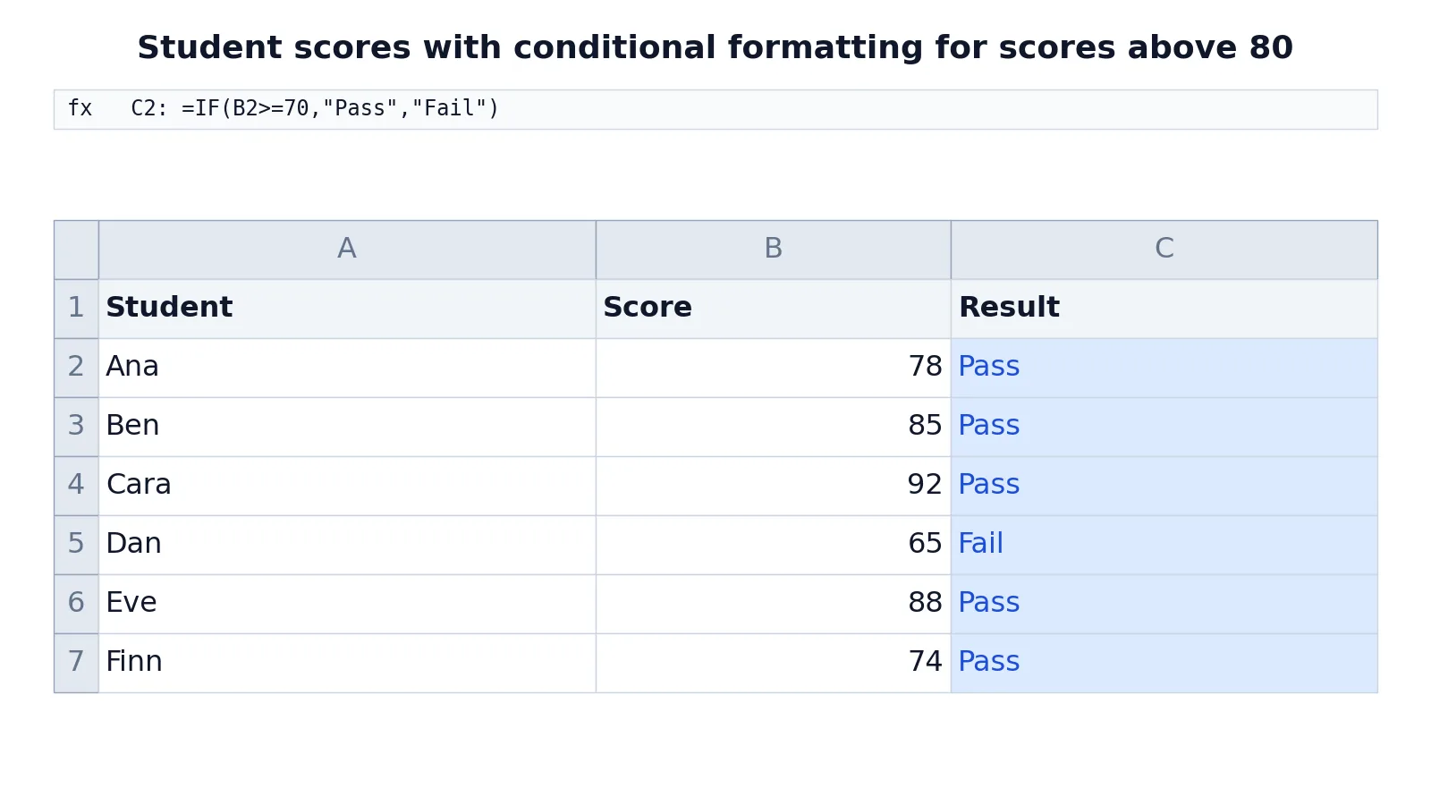
Take a small student score sheet. Column A holds names, column B holds scores, and column C uses an IF formula to mark Pass or Fail.

	A	B	C
1	Student	Score	Result
2	Ana	78	`=IF(B2>=70,"Pass","Fail")` -> displays Pass
3	Ben	85	`=IF(B3>=70,"Pass","Fail")` -> displays Pass
4	Cara	92	`=IF(B4>=70,"Pass","Fail")` -> displays Pass
5	Dan	65	`=IF(B5>=70,"Pass","Fail")` -> displays Fail
6	Eve	88	`=IF(B6>=70,"Pass","Fail")` -> displays Pass
7	Finn	74	`=IF(B7>=70,"Pass","Fail")` -> displays Pass

The IF rule in column C is the same formula copied down. In C2 it checks whether the score in B2 is at least 70 and shows Pass, otherwise Fail. The same rule copied down handles Ben in B3, Cara in B4, Dan in B5, Eve in B6, and Finn in B7. Dan's 65 is the only score below 70, so C5 is the only cell that displays Fail.

Now add a highlight rule on the scores:

Select B2:B7.
Go to Home > Conditional Formatting > Highlight Cells Rules > Greater Than...
Enter 80 in the dialog and choose Green Fill with Dark Green Text, then click OK.

After that, Ben (85), Cara (92), and Eve (88) are highlighted in green because their scores are above 80. Ana (78), Dan (65), and Finn (74) keep their normal formatting.

If you want to reproduce the same logic outside Excel, load the sheet with pandas and use numpy.where(df['Score'] > 80, 'green', 'none').

The figure below shows the result: scores above 80 are highlighted in green, and the Result column uses an IF formula to mark Pass or Fail.

Other Ways to Do It

Formula rules that reference another cell. This is the most flexible option. Select the cells you want to format, open New Rule, choose Use a formula to determine which cells to format, and write a formula that returns TRUE or FALSE [2][3]. For example, to highlight a whole row when the score in column B is above 80, select A2:C7 and use =$B2>80. The dollar sign locks the column so the rule always looks at column B, while the row number stays relative so each row is checked separately.

AND, OR, and NOT. You can combine conditions without wrapping them in IF. Excel supports AND, OR, and NOT directly in conditional formatting formulas [3]. For example, =AND($B2>80,$C2="Pass") highlights only rows that are both above 80 and marked Pass.

Banded rows. To shade alternate rows, use the formula =MOD(ROW(),2)=0 in a formula rule [6]. For alternate columns, use =MOD(COLUMN(),2)=0 [6].

Data bars, color scales, and icon sets. These compare values across a range at a glance. Data bars draw a bar whose length matches the value, color scales shade cells along a gradient, and icon sets assign one of three to five icons based on threshold values [5]. A three-icon set, for example, uses one icon for values at or above 67 percent, another for values below 67 percent and at or above 33 percent, and a third for values below 33 percent [5]. Icon sets can be combined with other conditional formats [5].

Google Sheets. The menu path differs. Select your range, then go to Format > Conditional formatting. The side panel opens with the same building blocks: a range, a format rule, and a format style. To format based on another cell, switch the rule to Custom formula is and write the formula the same way you would in Excel, such as =$B2>80.

Copying and clearing rules. To copy formatting, select a cell that already has the rule, click Format Painter, then select the cells you want to format [6]. To remove rules, select the cells and go to Home > Conditional Formatting > Clear Rules [4]. To remove all formatting, including non-conditional formats, go to Home > Clear > Clear Formats [6].

Troubleshooting

The format is not showing up. Check that the rule's range actually covers the cells you expect. Open Manage Rules and confirm the "Applies to" box [1].

The formula rule highlights the wrong cells. The formula is evaluated relative to the top-left cell of the selection. If you selected A2:C7 and wrote =B2>80, Excel shifts the reference for every row and column, which can produce unexpected results. Lock the column with $B2 when the condition should always read from one column.

A cell with an error is skipped. Conditional formatting is not applied to cells whose formula returns an error. Use IS or IFERROR to return a normal value instead [1].

Rules conflict. When two rules apply to the same cell, the one higher in the list wins if it sets the same format property. Reorder rules in Manage Rules to control which one takes priority [1].

Nothing happens after you type a value. Some rules only recalculate when the sheet recalculates. Press F9 to force a recalculation if a change is not reflected.

Common Mistakes

Writing a formula that returns a number instead of TRUE or FALSE. A formula rule needs a logical result. Wrap comparisons so the rule evaluates to TRUE or FALSE [2].
Forgetting the dollar sign. Without $B2, the column reference drifts as the rule is applied across columns. Lock the part that should stay fixed.
Selecting the wrong starting cell. The formula is written for the top-left cell of the selection. If you select B2:B7 but write the formula for B3, every row is off by one.
Applying a rule to the whole sheet by accident. Clicking the Select All button applies the rule everywhere, which slows large workbooks and produces odd results [6].
Stacking rules that fight each other. Two rules setting the same fill color create confusion. Use Manage Rules to check order and remove duplicates [1].
Expecting conditional formatting to change values. It only changes appearance. If you need the value itself to change, use a formula in the cell, as in the IF function guide.

Limitations

Conditional formatting is a display layer, so it does not alter, sort, or filter your underlying data. If you copy formatted cells to another program, the colors may not carry over, and if you export to CSV, all formatting is lost. Rules also do not travel well between Excel and Google Sheets, so a workbook moved between the two often needs its rules rebuilt.

Performance is the other constraint. Hundreds of formula rules across large ranges can slow a workbook noticeably, because Excel re-evaluates them on every recalculation. Keep rules scoped to the range that needs them, and prefer built-in rules over formula rules when a built-in rule does the same job. For related cleanup tasks, see how to highlight duplicates in Excel and how to filter in Excel once your rules are in place.

Frequently Asked Questions

How do I apply conditional formatting based on another cell in Excel?

Select the cells you want to format, open Home > Conditional Formatting > New Rule, and choose Use a formula to determine which cells to format [2]. Write a formula that references the other cell and returns TRUE or FALSE, such as =$B2>80. Lock the column with a dollar sign so the rule always reads from the same column while moving down the rows.

Can I use conditional formatting in Google Sheets the same way?

The logic is the same, but the menu is different. In Google Sheets, go to Format > Conditional formatting and use the side panel. For rules based on another cell, choose Custom formula is and write the formula exactly as you would in Excel.

Why is my conditional formatting not working?

The most common causes are a range that does not cover the cells, a formula written for the wrong starting cell, or a cell whose formula returns an error, since conditional formatting is skipped for error values [1]. Open Manage Rules and check the "Applies to" box first.

What is the difference between Highlight Cells Rules and a formula rule?

Highlight Cells Rules are presets for simple comparisons such as greater than, less than, or duplicate values [4]. A formula rule gives you full control and can reference other cells, combine conditions with AND, OR, and NOT, or format entire rows [3]. Use presets for speed and formulas for anything custom.

How do I remove conditional formatting?

Select the cells, then go to Home > Conditional Formatting > Clear Rules and pick the option you want [4]. To remove all formatting, including regular cell formats, use Home > Clear > Clear Formats [6]. To remove a single rule, open Manage Rules and delete it there [1].