Apriori Algorithm: Definition, Steps and Examples
By Dr. Zubair Khalid, DVM, MS, PhD ·
The apriori algorithm is a classic method for finding frequent itemsets and association rules in transaction data, such as market basket data. It works by counting how often combinations of items appear together, then pruning any combination that falls below a minimum support threshold. This article explains the definition, the step-by-step mechanics, and a fully worked example you can reproduce.
Quick Answer
- Apriori finds itemsets that appear together often enough in a set of transactions, then turns them into "if X then Y" rules.
- It uses two thresholds: minimum support (how often an itemset appears) and minimum confidence (how reliable a rule is).
- The core idea is the downward closure property: if an itemset is infrequent, every superset of it is also infrequent, so those candidates can be skipped.
- It proceeds level by level, first finding frequent single items, then frequent pairs, then triples, and so on.
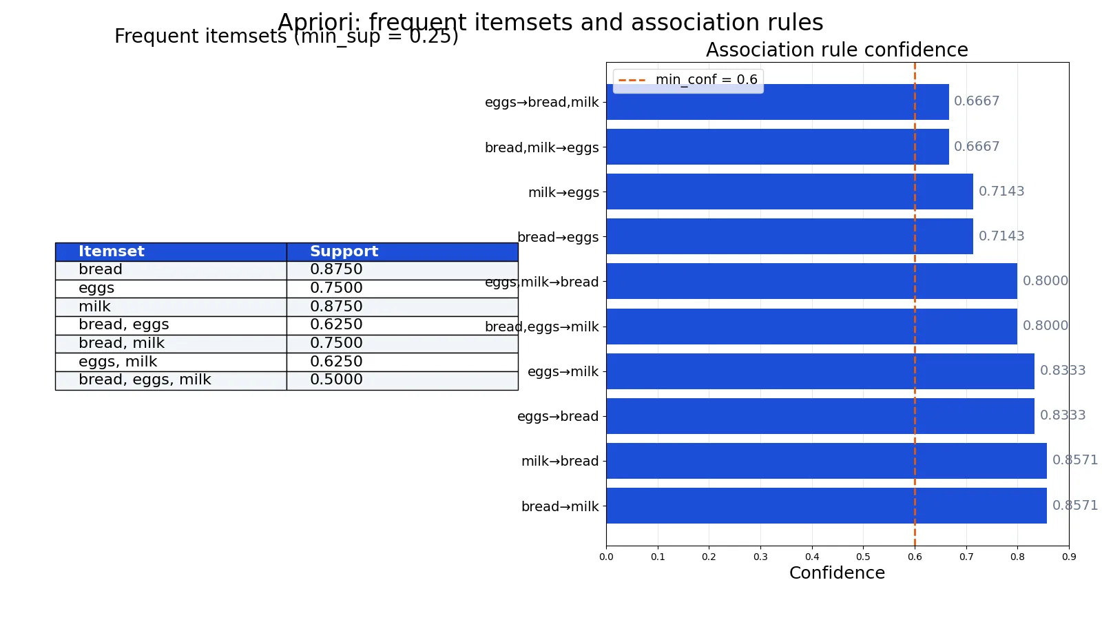
- In the worked example below, 8 transactions with a minimum support of 0.25 and minimum confidence of 0.6 produce 7 frequent itemsets and 10 rules.
What Apriori Means
In plain terms, apriori is a rule-mining algorithm that answers a simple question: which items tend to be bought or selected together? You give it a table of transactions, and it returns combinations of items that co-occur frequently, plus rules describing those co-occurrences.
The precise definition is narrower. Given a set of transactions $D$, where each transaction is a subset of items drawn from a universe $I$, apriori finds all itemsets $X \subseteq I$ whose support meets or exceeds a minimum support threshold. It then generates association rules $X \rightarrow Y$ from those frequent itemsets, keeping only rules whose confidence meets a minimum confidence threshold.
Two terms carry the whole method:
- Support of an itemset $X$ is the fraction of transactions that contain $X$.
- Confidence of a rule $X \rightarrow Y$ is the fraction of transactions containing $X$ that also contain $Y$.
The name comes from the fact that the algorithm uses prior knowledge of frequent itemset properties. Once you know an itemset is infrequent, you know a priori that no larger itemset containing it can be frequent.
How It Works
Apriori runs in two phases: find frequent itemsets, then generate rules from them.
Phase 1: Frequent itemset generation
The support of an itemset is:
$$\text{support}(X) = \frac{\text{count}(X)}{N}$$
where $\text{count}(X)$ is the number of transactions containing every item in $X$, and $N$ is the total number of transactions. An itemset is frequent when $\text{support}(X) \geq \text{min\_sup}$.
The algorithm builds itemsets level by level:
- Count single items. Scan the data and keep every item whose support passes the threshold. These are the frequent 1-itemsets.
- Join. Combine frequent 1-itemsets into candidate 2-itemsets.
- Prune. Remove any candidate that contains an infrequent subset. This is where the downward closure property saves work.
- Count and filter. Scan the data to get each candidate's support, and keep only those above the threshold.
- Repeat. Join the surviving $k$-itemsets into $(k+1)$-candidates, prune, count, and filter until no new candidates survive.
Phase 2: Rule generation
For each frequent itemset, split it into every possible antecedent $X$ and consequent $Y$. The confidence of a rule is:
$$\text{confidence}(X \rightarrow Y) = \frac{\text{support}(X \cup Y)}{\text{support}(X)}$$
Here $X \cup Y$ is the full itemset, and $X$ is the antecedent. A rule is kept when its confidence is at least $\text{min\_conf}$. Because every rule is built from a frequent itemset, its support is already known to pass the threshold.
Worked Example
The dataset is a small grocery log with 8 transactions and three items: bread, eggs, and milk. Each row is one item in one transaction.
| tid | item |
|---|---|
| 1 | bread |
| 1 | eggs |
| 1 | milk |
| 2 | bread |
| 2 | milk |
| 3 | bread |
| 3 | eggs |
| 4 | eggs |
| 4 | milk |
| 5 | bread |
| 5 | eggs |
| 5 | milk |
| 6 | bread |
| 6 | eggs |
| 6 | milk |
| 7 | bread |
| 7 | milk |
| 8 | bread |
| 8 | eggs |
| 8 | milk |
The parameters are $N = 8$ transactions, $\text{min\_sup} = 0.25$ (so an itemset needs a count of at least 2), and $\text{min\_conf} = 0.6$.
Step 1: Single-item support.
| Itemset | Count | Support |
|---|---|---|
| {bread} | 7 | 7/8 = 0.8750 |
| {eggs} | 6 | 6/8 = 0.7500 |
| {milk} | 7 | 7/8 = 0.8750 |
All three pass the 0.25 threshold.
Step 2: Pair support.
| Itemset | Count | Support |
|---|---|---|
| {eggs, bread} | 5 | 5/8 = 0.6250 |
| {milk, bread} | 6 | 6/8 = 0.7500 |
| {milk, eggs} | 5 | 5/8 = 0.6250 |
All three pairs pass.
Step 3: Triple support.
| Itemset | Count | Support |
|---|---|---|
| {milk, eggs, bread} | 4 | 4/8 = 0.5000 |
This passes too. There are no larger itemsets, so the algorithm stops with 7 frequent itemsets.
Step 4: Rule generation. Splitting each frequent itemset and applying the confidence formula gives 10 rules at or above 0.6:
| Rule | Support | Confidence |
|---|---|---|
| {bread} → {milk} | 0.75 | 0.7500 / 0.8750 = 0.8571 |
| {milk} → {bread} | 0.75 | 0.7500 / 0.8750 = 0.8571 |
| {eggs} → {bread} | 0.625 | 0.6250 / 0.7500 = 0.8333 |
| {eggs} → {milk} | 0.625 | 0.6250 / 0.7500 = 0.8333 |
| {eggs, bread} → {milk} | 0.5 | 0.5000 / 0.6250 = 0.8000 |
| {milk, eggs} → {bread} | 0.5 | 0.5000 / 0.6250 = 0.8000 |
| {bread} → {eggs} | 0.625 | 0.6250 / 0.8750 = 0.7143 |
| {milk} → {eggs} | 0.625 | 0.6250 / 0.8750 = 0.7143 |
| {milk, bread} → {eggs} | 0.5 | 0.5000 / 0.7500 = 0.6667 |
| {eggs} → {milk, bread} | 0.5 | 0.5000 / 0.7500 = 0.6667 |
Here is a compact Python version using an in-memory SQLite table to hold the transactions. The comments explain each stage.
import sqlite3, itertools

rows = [(1,'bread'),(1,'eggs'),(1,'milk'),(2,'bread'),(2,'milk'),(3,'bread'),(3,'eggs'),(4,'eggs'),(4,'milk'),(5,'bread'),(5,'eggs'),(5,'milk'),(6,'bread'),(6,'eggs'),(6,'milk'),(7,'bread'),(7,'milk'),(8,'bread'),(8,'eggs'),(8,'milk')]
con = sqlite3.connect(':memory:')
con.execute('CREATE TABLE transactions (tid INTEGER, item TEXT)')
con.executemany('INSERT INTO transactions VALUES (?,?)', rows)

N = 8
min_sup = 0.25
min_conf = 0.6

baskets = {}
for tid, item in rows:
    baskets.setdefault(tid, set()).add(item)

items = sorted({i for b in baskets.values() for i in b})
frequent = []
for k in range(1, len(items) + 1):
    for combo in itertools.combinations(items, k):
        s = set(combo)
        count = sum(1 for b in baskets.values() if s <= b)
        if count / N >= min_sup:
            frequent.append((s, count / N))

rules = []
for s, sup in frequent:
    for r in range(1, len(s)):
        for ant in itertools.combinations(s, r):
            ant = set(ant)
            con_ = s - ant
            conf = sup / (sum(1 for b in baskets.values() if ant <= b) / N)
            if conf >= min_conf:
                rules.append((ant, con_, sup, conf))

rules.sort(key=lambda r: -r[3])
print(f"Frequent itemsets: {len(frequent)}; rules: {len(rules)}")
for ant, cons, sup, conf in rules:
    print(f"{ant} -> {cons}  conf={conf:.4f}")
Output:
Frequent itemsets: 7; rules: 10
{'bread'} -> {'milk'}  conf=0.8571
{'milk'} -> {'bread'}  conf=0.8571
{'eggs'} -> {'bread'}  conf=0.8333
{'eggs'} -> {'milk'}  conf=0.8333
{'eggs', 'bread'} -> {'milk'}  conf=0.8000
{'milk', 'eggs'} -> {'bread'}  conf=0.8000
{'bread'} -> {'eggs'}  conf=0.7143
{'milk'} -> {'eggs'}  conf=0.7143
{'milk', 'bread'} -> {'eggs'}  conf=0.6667
{'eggs'} -> {'milk', 'bread'}  conf=0.6667
If you want to build up the surrounding data skills first, the Python for machine learning guide covers the tooling you need for this kind of counting work.
How to Interpret It
Support tells you how common an itemset is. A support of 0.75 for {milk, bread} means three-quarters of all transactions contain both. Low support means the pattern is rare, and rare patterns are often noise in small datasets.
Confidence tells you how dependable a rule is. The rule {bread} → {milk} has confidence 0.8571, so when bread appears, milk appears about 86 percent of the time. Confidence is directional: {bread} → {milk} and {milk} → {bread} can have different values, though in this dataset they happen to match because both items have the same support.
Read the two numbers together. A rule with high confidence but low support describes a pattern that is reliable when it happens but rarely happens. A rule with high support but low confidence describes a common combination that is not a strong predictor. The most useful rules usually clear both thresholds.
When to Use It (and when not to)
Use apriori when your data is naturally a set of transactions or baskets, when you want human-readable rules, and when the item universe is modest. Typical cases include retail market basket analysis, cross-sell recommendations, web clickstream patterns, and finding co-occurring symptoms or codes in event logs.
Do not reach for it when you need prediction accuracy on a labeled target. Apriori describes co-occurrence, it does not build a classifier. If your goal is to predict a class from features, a probabilistic classifier such as Naive Bayes is a better fit.
Also avoid it when the item universe is very large and dense. The number of candidate itemsets grows quickly, and the repeated scans become expensive. In those settings, alternatives that avoid candidate generation are usually preferred.
Apriori vs Frequent Pattern Growth
Frequent pattern growth (FP-growth) is the closest alternative. It compresses the data into a tree structure and mines patterns from that tree without generating candidate itemsets.
| Aspect | Apriori | FP-growth |
|---|---|---|
| Core mechanism | Candidate generation and pruning | Tree compression, no candidates |
| Database scans | Multiple, one per level | Typically two |
| Speed on dense data | Slower | Usually faster |
| Output | Frequent itemsets and rules | Same frequent itemsets and rules |
| Interpretability | Step-by-step, easy to trace | Harder to trace by hand |
Both produce the same frequent itemsets for the same thresholds. The difference is efficiency, not results.
Common Mistakes
- Setting minimum support too low. You get thousands of itemsets, most of them meaningless. Fix: raise the threshold until the output is small enough to inspect, then lower it gradually.
- Setting minimum support too high. You miss real patterns because nothing clears the bar. Fix: check the support distribution of single items first and pick a threshold near the low end of what is common.
- Treating confidence as causation. A high-confidence rule means co-occurrence, not that one item causes the other. Fix: describe rules as associations and validate any causal claim with a controlled test.
- Ignoring the direction of a rule. {bread} → {milk} and {milk} → {bread} are different rules with potentially different confidence. Fix: always report the antecedent and consequent explicitly.
- Forgetting that support is relative to N. The same count means different support in datasets of different sizes. Fix: state $N$ alongside every support value.
- Mining itemsets with no business meaning. Rare or trivially related items can dominate the output. Fix: filter items before mining and review rules with a domain expert.
Limitations
Apriori cannot tell you whether an association is useful or causal. It reports patterns that meet your thresholds, and those thresholds are choices you make. Change them and the rule set changes. A rule that looks strong in a small dataset may be an artifact of a handful of transactions, so support values from small samples deserve caution.
The algorithm also scales poorly in some conditions. When transactions are long and the item universe is large, the number of candidate itemsets can explode, and each level requires another pass over the data. Memory and runtime can become the binding constraint long before you reach an interesting result. For very large or dense datasets, consider FP-growth or a constraint-based approach.
Frequently Asked Questions
What is the difference between support and confidence?
Support measures how often an itemset appears in the whole dataset. Confidence measures how often the consequent appears among the transactions that contain the antecedent. Support is symmetric for an itemset, confidence is directional for a rule.
Does apriori need a minimum support threshold?
Yes. The threshold is what makes the search tractable. Without it, every possible itemset would be a candidate, and the downward closure pruning would have nothing to remove. You can also set a minimum confidence to filter the rules after mining.
Can apriori handle more than three items?
Yes. The worked example stops at three items only because the dataset has three distinct items. The algorithm continues joining and pruning until no candidate itemset survives, so it handles any itemset size your data supports.
Why is apriori slow on large datasets?
It scans the transaction data once per itemset size, and the number of candidate itemsets can grow very large before pruning takes effect. Both the repeated scans and the candidate explosion add cost as the item universe and transaction length increase.
What should I use instead of apriori?
FP-growth is the common replacement because it avoids candidate generation and usually needs fewer passes over the data. If you need prediction rather than pattern discovery, use a supervised classifier instead.
References
This article draws on the standard references listed under Further Reading.
Further Reading
- Lever J, Krzywinski M, Altman N (2016). Classification evaluation. Nature Methods
- scikit-learn User Guide
- Wilson G, Bryan J, Cranston K et al. (2017). Good enough practices in scientific computing. PLOS Computational Biology
- Lever J, Krzywinski M, Altman N (2016). Model selection and overfitting. Nature Methods
- Saito T, Rehmsmeier M (2015). The Precision-Recall Plot Is More Informative than the ROC Plot When Evaluating Binary Classifiers on Imbalanced Datasets. PLOS ONE
- NIST/SEMATECH e-Handbook of Statistical Methods