Excel Formulas Cheat Sheet: Key Functions and Examples
By Dr. Zubair Khalid, DVM, MS, PhD ·
If you want a fast reference for the functions you use most, this excel cheat sheet formulas guide covers syntax, arguments and short examples you can copy into your own workbook. Each entry shows what the function does, what it returns, and where it goes wrong. Keep it open beside your spreadsheet while you work.
Quick Answer
- Every formula starts with
=and returns a single value in the cell that holds it. - Core math functions are
SUM,AVERAGE,MIN,MAXandCOUNT, all of which accept ranges likeA1:A10. - Logical tests use
IF(condition, value_if_true, value_if_false)and can be nested. - Lookups use
VLOOKUP(lookup_value, table_array, col_index_num, range_lookup)to pull a value from another column. - Parentheses control the order of operations, so
=(A1+B1)*C1differs from=A1+B1*C1[1].
What Excel Formulas Mean
A formula is an instruction that tells Excel to calculate something and display the result in the cell. The formula itself lives in the formula bar, while the cell shows the outcome. That separation matters because you edit the logic, not the number.
The precise definition is narrower. A formula is an expression beginning with an equals sign that combines operators, cell references, constants and functions to produce a value. Operators include +, -, * and /. Cell references point to other cells, such as B2 or $C$2. Functions are named procedures that take arguments in parentheses and return a result.
Excel evaluates formulas using standard arithmetic precedence. Multiplication and division happen before addition and subtraction, and parentheses override that order. Brackets in formulas are not decorative, they change which operations are grouped together and therefore change the answer [1].
If you are new to the topic, start with Excel formula basics before memorizing individual functions.
How It Works
Every function follows the same shape:
$$=\text{FUNCTION}(\text{argument1}, \text{argument2}, \dots)$$
Each symbol has a job.
=marks the start of the formula.FUNCTIONis the name, such asSUMorIF.(and)enclose the arguments.,separates one argument from the next.argumentis a value, a cell reference, a range or another formula.
A range like $C$2:$C$5 refers to a block of cells. The dollar signs lock the reference so it does not shift when you copy the formula down. Without them, C2:C5 becomes C3:C6 on the next row, which is often what you want and sometimes is not.
For a full tour of the building blocks, see the Excel functions overview.
Worked Example
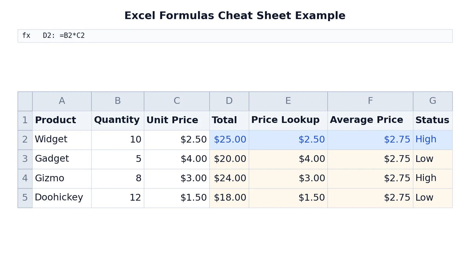
The sheet below tracks four products with quantity, unit price, a calculated total, a price lookup, an average price and a status label.
| A | B | C | D | E | F | G | |
|---|---|---|---|---|---|---|---|
| 1 | Product | Quantity | Unit Price | Total | Price Lookup | Average Price | Status |
| 2 | Widget | 10 | 2.5 | =B2*C2 -> displays $25.00 | =VLOOKUP(A2,$A$2:$C$5,3,FALSE) -> displays $2.50 | =AVERAGE($C$2:$C$5) -> displays $2.75 | =IF(D2>20,"High","Low") -> displays High |
| 3 | Gadget | 5 | 4 | =B3*C3 -> displays $20.00 | =VLOOKUP(A3,$A$2:$C$5,3,FALSE) -> displays $4.00 | =AVERAGE($C$2:$C$5) -> displays $2.75 | =IF(D3>20,"High","Low") -> displays Low |
| 4 | Gizmo | 8 | 3 | =B4*C4 -> displays $24.00 | =VLOOKUP(A4,$A$2:$C$5,3,FALSE) -> displays $3.00 | =AVERAGE($C$2:$C$5) -> displays $2.75 | =IF(D4>20,"High","Low") -> displays High |
| 5 | Doohickey | 12 | 1.5 | =B5*C5 -> displays $18.00 | =VLOOKUP(A5,$A$2:$C$5,3,FALSE) -> displays $1.50 | =AVERAGE($C$2:$C$5) -> displays $2.75 | =IF(D5>20,"High","Low") -> displays Low |
Four formulas do the work.
D2 multiplies quantity by unit price to get the total. The result is $25.00.
E2 looks up the unit price for the product named in column A. It searches the range $A$2:$C$5, takes the value from the third column of that range, and requires an exact match because the last argument is FALSE. The result is $2.50.
F2 calculates the average unit price across all four products. The result is $2.75, and it stays the same on every row because the range is locked.
G2 returns "High" if the total exceeds 20, otherwise "Low". The result is High.
The figure below shows the same layout. A sample sheet demonstrating SUM, AVERAGE, IF, and VLOOKUP with product data.
How to Interpret It
Read a formula result in context, not in isolation. The total in column D is a per-row calculation, so each row answers a different question. The average in column F is a fixed reference point, so comparing a row total against it tells you whether that product is above or below the typical price.
The lookup in column E is a retrieval, not a calculation. If it returns a value, the product name exists in the lookup range. If it returns an error, the name does not match exactly, which is usually a spelling or spacing problem.
The status in column G turns a number into a category. Once you have categories, you can count them with COUNTIF, which is often more useful than reading individual rows. For counting patterns generally, see COUNT function in Excel.
When to Use It (and when not to)
Use these functions when your data is tabular, one record per row, and the calculation logic is the same on every row. That covers most reporting, budgeting and tracking work.
Use SUM and AVERAGE when you need a single summary number. Use IF when a decision depends on a threshold. Use VLOOKUP when you need to pull a matching value from a reference table.
Avoid VLOOKUP when the value you want sits to the left of the lookup column. It cannot look backwards. Use INDEX with MATCH instead, or restructure the table. Avoid AVERAGE when your range contains zeros that mean "no data" rather than "zero value", because those zeros pull the average down. Avoid hard-coded numbers inside formulas when the value might change, since you will have to hunt through every formula to update it.
SUM vs AVERAGE
These two are often confused because both summarize a range, but they answer different questions.
| SUM | AVERAGE | |
|---|---|---|
| Question answered | What is the total? | What is the typical value? |
| Syntax | =SUM(range) | =AVERAGE(range) |
| Sensitive to outliers | Yes, one large value changes it | Less so, but still affected |
| Ignores blank cells | Yes | Yes |
| Counts text cells | No | No |
| Typical use | Totals, budgets, quantities | Benchmarks, comparisons |
Use SUM when the total itself is the answer. Use AVERAGE when you need a baseline to compare individual values against.
Common Mistakes
- Forgetting the equals sign. Without
=, Excel treats the entry as text and shows it literally. Add=at the start. - Mixing relative and absolute references. Copying
=B2*C2down is fine, but copying a lookup range without$shifts it and breaks the match. Lock the range with$A$2:$C$5. - Using the wrong final argument in
VLOOKUP.TRUEallows an approximate match and can return a wrong value from an unsorted table. UseFALSEfor exact matches. - Ignoring operator precedence.
=A1+B1*C1multiplies first. Wrap the addition in parentheses if you want it done first [1]. - Leaving unmatched parentheses. Excel flags the error, but long nested formulas hide the problem. Count the opening and closing brackets.
- Averaging a range that includes totals. If a total row sits inside your range,
AVERAGEincludes it and inflates the result. Exclude summary rows from the range.
Limitations
These functions work on values, not on meaning. VLOOKUP ignores case but not spaces, so "Widget" and "widget " with a trailing space are different values and the lookup fails. IF handles one condition cleanly, but stacking many conditions makes a formula hard to read and hard to debug.
AVERAGE and SUM ignore text and blank cells, which is usually helpful but can hide gaps in your data. A column where half the prices are missing still returns an average, and that average may not represent anything real. Always check how many values went into a calculation before trusting the result.
Frequently Asked Questions
What is the difference between a formula and a function?
A formula is any expression that starts with = and produces a value. A function is a named procedure inside a formula, such as SUM or IF. Every function is used within a formula, but not every formula contains a function. =A1+B1 is a formula with no function at all.
Why does my VLOOKUP return #N/A?
The lookup value was not found in the first column of your range. Common causes are trailing spaces, numbers stored as text, or a lookup range that does not include the row you expect. Capitalization is not a cause, because VLOOKUP ignores case. Check the exact text in both places.
How do I average only some of the values in a range?
Use AVERAGEIF or AVERAGEIFS to apply a condition. For example, =AVERAGEIF(B2:B5,">6") averages only the values above 6. Plain AVERAGE includes every numeric cell in the range with no filtering.
Can I put a formula inside another formula?
Yes. This is called nesting, and it is common with IF. Keep nesting shallow, two or three levels at most, because deeper nesting becomes difficult to read and to correct. If you need many conditions, consider a lookup table instead.
How do I round a calculated result?
Wrap the calculation in ROUND. For example, =ROUND(B2*C2,2) rounds the total to two decimal places. The second argument is the number of digits. See the Excel ROUND function for more detail, and Excel SUM function examples for more on aggregation.
References
Further Reading
- Broman KW, Woo KH (2018). Data Organization in Spreadsheets. The American Statistician
- Ziemann M, Eren Y, El-Osta A (2016). Gene name errors are widespread in the scientific literature. Genome Biology
- Microsoft Support: Excel help and learning
- McCullough B, Heiser DA (2008). On the accuracy of statistical procedures in Microsoft Excel 2007. Computational Statistics & Data Analysis
- Abeysooriya M, Soria M, Kasu MS et al. (2021). Gene name errors: Lessons not learned. PLOS Computational Biology