Critical Value Table: How to Read and Use One

By Dr. Zubair Khalid, DVM, MS, PhD · 2026-10-03

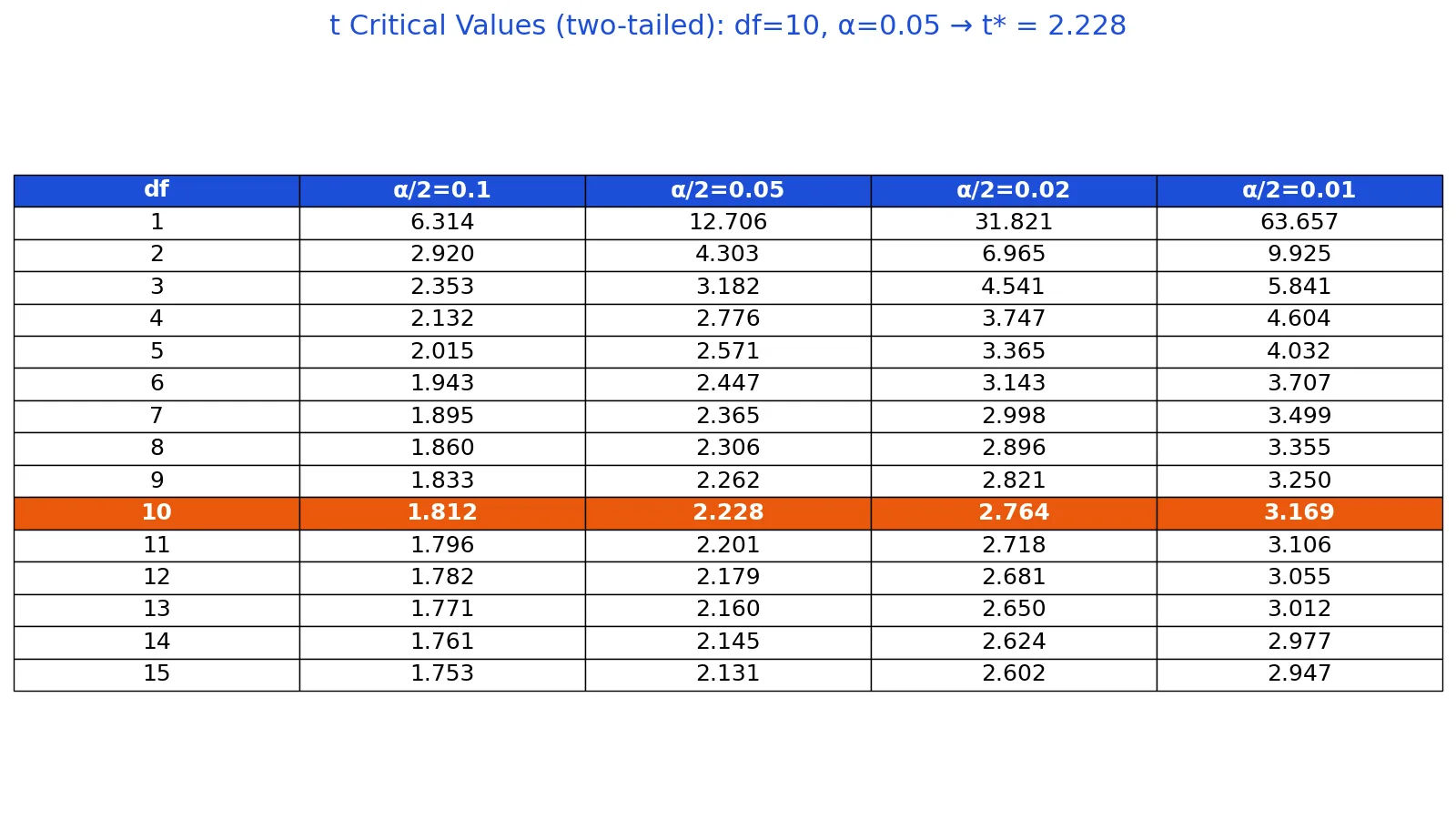
A critical value table is a precomputed grid of cutoff numbers for a test statistic. You look up one value using your significance level and degrees of freedom, then compare it with the statistic you calculated from your data. If your statistic is more extreme than the table value, you reject the null hypothesis.

Quick Answer

A critical value table lists cutoffs for a test statistic at common significance levels, usually $\alpha = 0.10$, $0.05$ and $0.01$ [1].
The table value depends on the test statistic, the significance level $\alpha$, and the degrees of freedom [1].
You read the table by finding the row for your degrees of freedom and the column for your $\alpha$ or confidence level [2].
For a two-sided test, split $\alpha$ across both tails, so you look up $1 - \alpha/2$ [2].
Reject the null hypothesis when the absolute value of your test statistic is greater than the critical value [2].

What a Critical Value Table Means

In plain terms, a critical value table is a lookup chart. Instead of computing a cutoff from a formula every time, you read it off a printed or online grid. The table tells you how far a statistic has to stray from what the null hypothesis predicts before you call the result statistically significant.

The precise definition: a critical value is the boundary of a rejection region, the set of test statistic values that are unlikely to occur when the null hypothesis is true [1]. The significance level $\alpha$ is the probability of landing in that region when the null is actually true, so a test at $\alpha = 0.05$ rejects a true null hypothesis 5% of the time [1]. Because each test statistic has its own distribution, there is a separate critical value table for each one, including t, chi-square and F [1].

How It Works

Every critical value table encodes the same idea. You pick a tail probability, find the point on the distribution that cuts off that probability, and compare your statistic with it.

For a statistic $T$ with a known distribution under the null hypothesis, the critical value $t^*$ satisfies:

$$P(T > t^* \mid H_0) = \alpha$$

Each symbol means the following:

$T$ is the test statistic computed from your sample, such as a t statistic or a chi-square statistic.
$t^*$ is the critical value you read from the table.
$\alpha$ is the significance level, the tail probability you are willing to accept as a false positive [1].
$H_0$ is the null hypothesis, the default claim you are testing against.

The decision rule follows directly. For an upper one-sided t test, reject $H_0$ when the statistic exceeds the table value. For a lower one-sided test, reject when it falls below the negative of the table value. For a two-sided test, reject when the absolute value exceeds the value in the $1 - \alpha/2$ column [2].

The same logic drives other tables. The chi-square distribution is not symmetric, so it has separate upper-tail and lower-tail tables, and a two-sided test compares the statistic against both [3]. The F table is built from upper critical values indexed by numerator and denominator degrees of freedom [4].

Worked Example

The dataset below records systolic blood pressure in mmHg before and after a 6-week intervention for 11 clinic patients. The question is whether the mean change differs from zero.

patient_id	before	after	difference
1	142	138	4
2	138	134	4
3	145	140	5
4	150	146	4
5	136	133	3
6	148	143	5
7	141	137	4
8	139	136	3
9	147	142	5
10	143	139	4
11	140	137	3

The steps run as follows.

Sample size: $n = 11$.
Differences (before minus after): 4, 4, 5, 4, 3, 5, 4, 3, 5, 4, 3.
Mean difference: $44 / 11 = 4.0000$.
Sample standard deviation: $sd = 0.7746$.
Standard error: $SE = 0.7746 / \sqrt{11} = 0.2335$.
t statistic: $t = 4.0000 / 0.2335 = 17.1270$.
Degrees of freedom: $df = n - 1 = 10$.
Two-tailed critical value: $t^* = 2.2281$ at $\alpha = 0.05$.
Decision: $|t| = 17.1270 > 2.2281$, so reject $H_0$.
p-value: $p = 0.0000$.

Here is the same calculation in code.

from scipy import stats
t_stat = 17.1270
t_crit = stats.t.ppf(1 - 0.05/2, 10)  # 2.2281
p = 2 * (1 - stats.t.cdf(abs(t_stat), 10))  # 0.0000

Output:

t = 17.1270, t* = 2.2281, p = 0.0000 -> reject H0

The computed t of 17.1270 sits far beyond the critical value of 2.2281, so the mean drop in blood pressure is statistically significant at the 5% level. If you want the full mechanics of this table, see Understanding the t-Test Table: How to Use It for Significance.

How to Interpret It

Reading the table gives you one number. Interpreting it means asking how far your statistic sits from that number.

A statistic just past the critical value is barely significant. A statistic far past it, like 17.1270 against 2.2281, is significant by a wide margin. The critical value itself does not measure effect size. It only marks the boundary where chance alone becomes an unlikely explanation.

The critical value and the p-value always agree. Rejecting when $|t| > t^*$ is the same decision as rejecting when $p < \alpha$ [1]. If your software reports a p-value, you rarely need the table, but the table helps you see why the decision came out the way it did.

When to Use It (and when not to)

Use a critical value table when you are running a hypothesis test by hand, when you are teaching or learning the logic of rejection regions, or when your software does not report a p-value. It is also useful when you want a fixed decision rule before you see the data, which is good practice [1].

Skip the table when your software already returns a p-value and a confidence interval. Skip it when your test statistic does not follow a standard distribution, since the table only covers the distributions it was built for. For chi-square work, use a dedicated Chi-Square Table: How to Read It and Find Critical Values. For variance comparisons across groups, use the F Distribution Table: How to Read and Use It. For proportions and z tests, see How to Find the Critical Z Value (With Examples).

Critical Value Table vs p-Value

Both approaches answer the same question, but they present the answer differently.

Feature	Critical value table	p-value
What it gives you	A cutoff for the test statistic	The probability of a result at least as extreme as yours [1]
Decision rule	Reject when the statistic exceeds the cutoff [2]	Reject when $p < \alpha$ [1]
Needs degrees of freedom	Yes, to pick the row [2]	Handled internally by software
Best for	Hand calculations and teaching	Reporting results in papers
Agreement	Always matches the p-value decision [1]	Always matches the table decision [1]

Common Mistakes

Using the wrong tail column. For a two-sided test at $\alpha = 0.05$, look up $1 - \alpha/2 = 0.975$, not $0.95$ [2]. Fix: decide one-sided or two-sided before you open the table.
Forgetting to take the absolute value. A large negative t statistic is just as significant as a large positive one. Fix: compare $|t|$ with the critical value for two-sided tests [2].
Using the wrong degrees of freedom. For a paired t test, $df = n - 1$. For a two-sample test, the formula differs. Fix: confirm the df formula for your specific test.
Reading a chi-square upper-tail value for a lower-tail test. The chi-square distribution is not symmetric, so the two tails have separate tables [3]. Fix: match the table to the direction of your test.
Treating the critical value as an effect size. A significant result is not automatically a large or important one. Fix: report a confidence interval or effect size alongside the decision.
Mixing tables from different sources. Versions of the same table can differ slightly in rounding [5]. Fix: use one consistent table throughout an analysis.

Limitations

A critical value table only covers the significance levels and degrees of freedom that were printed. If your $\alpha$ or df falls between listed values, you cannot read an exact cutoff, and you may need interpolation or software. The table also assumes your test statistic follows the named distribution, which depends on assumptions like normality or equal variances holding in your data.

The table gives a binary decision and nothing more. It does not tell you how large an effect is, how precise your estimate is, or whether the result matters in practice. A statistically significant result from a huge sample can be trivial in size, and the table will not warn you about that.

Frequently Asked Questions

What is a critical value table used for?

It provides the cutoff a test statistic must exceed for you to reject the null hypothesis at a chosen significance level [1]. You use it in hypothesis testing when you want a fixed decision rule or when you are working by hand.

How do I read a critical value table?

Find the row for your degrees of freedom and the column for your significance level or confidence level [2]. The cell where they meet is your critical value. For two-sided tests, use the $1 - \alpha/2$ column [2].

What is the difference between a one-tailed and two-tailed critical value?

A one-tailed test puts all of $\alpha$ in one tail, so you look up $1 - \alpha$. A two-tailed test splits $\alpha$ across both tails, so you look up $1 - \alpha/2$, which gives a larger critical value [2].

Why does the critical value change with degrees of freedom?

The shape of the t distribution depends on the sample size through the degrees of freedom. With few degrees of freedom the tails are heavier, so the critical value is larger. As df grows, the t distribution approaches the normal distribution and the critical value shrinks toward the z value [2].

Can I use a critical value table instead of a p-value?

Yes, the two always lead to the same decision [1]. Rejecting when the statistic exceeds the critical value is equivalent to rejecting when the p-value is below $\alpha$. Many researchers report the p-value because it carries more information about how extreme the result is.

References

7.1.3.1. Critical values and p values
1.3.6.7.2. Critical Values of the Student's-t Distribution
1.3.6.7.4. Critical Values of the Chi-Square Distribution
2.3.6.5.3. Table of critical values of F distribution
Common Critical Value Tables - Statistics LibreTexts_WITHOUT_UNITS/zz%3A_Back_Matter/02%3A_Common_Critical_Value_Tables)