How to Find the Critical Z Value (With Examples)

By Dr. Zubair Khalid, DVM, MS, PhD · 2026-10-03

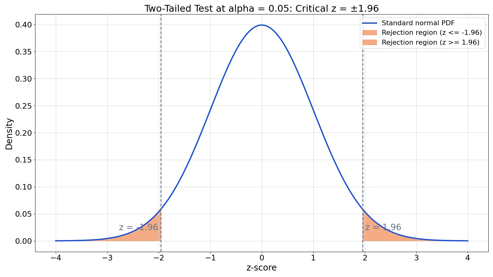
To find the critical z value, you work backward from the significance level $\alpha$ using the standard normal distribution. For a two-tailed test at $\alpha = 0.05$, the critical values are $\pm 1.96$. For a one-tailed test at the same level, the critical value is $1.6449$ on the right or $-1.6449$ on the left. This article shows how to find critical z values step by step, with a worked example and the tools that do the arithmetic for you.

Quick Answer

A critical z value is the cutoff on the standard normal curve where the rejection region begins [1].
Two-tailed test at $\alpha = 0.05$: $z = \pm 1.96$ [2].
One-tailed test at $\alpha = 0.05$: $z = 1.6449$ (right) or $-1.6449$ (left).
The formula uses the inverse normal CDF: two-tailed $z = \Phi^{-1}(1 - \alpha/2)$, one-tailed $z = \Phi^{-1}(1 - \alpha)$.
In Excel, =NORM.S.INV(1-0.05/2) returns 1.9600.

Before You Start

You need three things before you look up a z value.

First, the significance level $\alpha$. Common choices are 0.10, 0.05, and 0.01 [1]. This is the probability of rejecting the null hypothesis when it is actually true, so a smaller $\alpha$ means a stricter test and a larger critical value.

Second, the direction of the test. A two-tailed test splits $\alpha$ between both ends of the curve. A one-tailed test puts all of $\alpha$ in one tail, either the right or the left.

Third, the standard normal distribution. The z distribution has a mean of 0 and a standard deviation of 1. Critical values come from this distribution, not from your sample. That is what separates a z-test from a t-test, whose critical values depend on the sample size through the degrees of freedom [2].

If you also need cutoffs for other test statistics, the same logic applies to the chi-square distribution, which you can read about in this guide to the chi-square table.

Step by Step

State your significance level. Write down $\alpha$. For this walkthrough, use $\alpha = 0.05$.

Decide one-tailed or two-tailed. This comes from your alternative hypothesis. "Not equal to" is two-tailed. "Greater than" or "less than" is one-tailed.

Compute the cumulative probability. For a two-tailed test, the cumulative probability at the upper cutoff is $1 - \alpha/2$, leaving $\alpha/2$ in the upper tail. For a one-tailed right test, it is $1 - \alpha$. For a one-tailed left test, it is $\alpha$.

Apply the inverse normal CDF. The critical value is the z-score whose cumulative probability equals the tail probability you just computed.

$$z_{\text{two-tailed}} = \Phi^{-1}\!\left(1 - \frac{\alpha}{2}\right)$$

$$z_{\text{one-tailed right}} = \Phi^{-1}(1 - \alpha)$$

Attach the sign. The right tail is positive. The left tail is negative. A two-tailed test uses both signs.

Compare your test statistic to the critical value. Reject the null hypothesis when the test statistic falls in the rejection region beyond the critical value [1].

Here is the full set of values at the three most common significance levels.

Test type	$\alpha = 0.10$	$\alpha = 0.05$	$\alpha = 0.01$
Two-tailed	$\pm 1.6449$	$\pm 1.9600$	$\pm 2.5758$
One-tailed (right)	$1.2816$	$1.6449$	$2.3263$
One-tailed (left)	$-1.2816$	$-1.6449$	$-2.3263$

A critical value table lists these same cutoffs if you prefer reading values instead of computing them.

Worked Example

The dataset is a set of quiz scores from a class of 15 students, used here to set up a one-sample z-test against a hypothesized mean.

student_id	score
1	72
2	85
3	90
4	68
5	77
6	81
7	95
8	64
9	88
10	79
11	83
12	70
13	92
14	75
15	86

The summary statistics come out as follows.

Step	Value
Sample size $n$	15
Sample mean	80.3333
Sample standard deviation ($n-1$)	9.2633
Significance level $\alpha$	0.05
Two-tailed cumulative probability	$1 - \alpha/2 = 0.9750$
Two-tailed critical z	$\Phi^{-1}(0.9750) = 1.9600$
One-tailed right cumulative probability	$1 - \alpha = 0.9500$
One-tailed right critical z	$\Phi^{-1}(0.9500) = 1.6449$
One-tailed left critical z	$\Phi^{-1}(0.0500) = -1.6449$

The code below reproduces every number.

from scipy import stats
alpha = 0.05
z_two = stats.norm.ppf(1 - alpha/2)   # two-tailed
z_one = stats.norm.ppf(1 - alpha)     # one-tailed right
print(f"Two-tailed critical z = {z_two:.4f}; one-tailed (right) critical z = {z_one:.4f}; one-tailed (left) critical z = {-z_one:.4f}")

Output:

Two-tailed critical z = 1.9600; one-tailed (right) critical z = 1.6449; one-tailed (left) critical z = -1.6449

So if your alternative hypothesis is "the mean is not equal to the hypothesized value," you reject the null when your z statistic is above 1.96 or below -1.96. If your alternative is "the mean is greater," you reject when the statistic exceeds 1.6449.

Other Ways to Do It

Excel. =NORM.S.INV(1-0.05/2) returns 1.9600. For a one-tailed right test, use =NORM.S.INV(1-0.05), which returns 1.6449. The function takes a cumulative probability between 0 and 1 and returns the corresponding z-score.

A z table. Standard normal tables list cumulative probabilities for z-scores to two decimal places [3]. Find the probability closest to your target tail probability, then read the z-score from the row and column headers. Tables give you about two decimal places of precision, which is enough for most classroom work.

A critical z value calculator. Any tool that computes the inverse normal CDF does the job. You enter $\alpha$ and the number of tails, and it returns the cutoff. This is the fastest route when you already know your test setup.

Statistical software. Python's scipy.stats.norm.ppf, R's qnorm, and most stats packages expose the same inverse CDF. The argument is always a cumulative probability.

If your test involves two proportions instead of a mean, the critical z value works the same way, and the two proportion z-test formula shows how the statistic is built.

Troubleshooting

You got a negative value for a right-tailed test. You passed $\alpha$ instead of $1 - \alpha$ to the inverse CDF. The right tail always uses a probability above 0.5.

Your value is close to but not exactly 1.96. That is rounding. The true value is 1.959964, which rounds to 1.96. Tables and most software report 1.96 [2].

You cannot decide between one and two tails. Look at your alternative hypothesis, not your data. Choosing the tail after seeing the results inflates your false positive rate.

Your software asks for a probability and you gave it a percentage. Enter 0.05, not 5.

You are unsure whether to use z or t. Use z when you know the population standard deviation. Use t when you only have the sample standard deviation, since t critical values depend on the sample size [2].

Common Mistakes

Splitting alpha for a one-tailed test. A one-tailed test puts the whole $\alpha$ in one tail. Splitting it gives you the two-tailed cutoff and makes the test harder to pass than intended. Fix: use $1 - \alpha$ for a one-tailed right test.
Using the sample standard deviation with a z critical value. The z-test assumes you know the population standard deviation [2]. If you substituted the sample value, a t critical value is the correct choice.
Reading the table's body as the z-score. In a standard normal table, the body holds probabilities and the margins hold z-scores [3]. Reading them backward gives nonsense. Fix: locate your probability in the body first.
Forgetting the sign on the left tail. The left critical value is negative. Comparing a negative test statistic to a positive cutoff flips your conclusion.
Picking alpha after running the test. The significance level belongs in your analysis plan before you see data [1]. Changing it afterward turns a null result into a "significant" one.
Confusing the critical value with the p-value. The critical value is a cutoff on the z scale. The p-value is a probability. They answer the same question from opposite directions [1].

Limitations

The critical z value approach assumes the test statistic follows a standard normal distribution under the null hypothesis. That assumption holds well for large samples by the central limit theorem, but it can fail for small samples from skewed or heavy-tailed populations. In those cases the nominal $\alpha$ is not the true rejection rate, and your conclusions can be off even though the arithmetic is correct.

The method also says nothing about practical importance. A result can clear the critical value and still be too small to matter, especially with a large sample where tiny effects become statistically detectable. The critical value is a decision rule, not a measure of how much the effect matters. For a broader view of how cutoffs work across distributions, see how to find Q1 and Q3 for the quantile logic behind these values.

Frequently Asked Questions

What is the critical z value for a 95% confidence level?

For a two-tailed test at $\alpha = 0.05$, the critical values are $\pm 1.96$ [2]. The 95% refers to the confidence level, which is $1 - \alpha$. The same 1.96 appears in confidence intervals for a mean when the population standard deviation is known.

How do I find the critical z value for a two-tailed test?

Divide $\alpha$ by 2, subtract that from 1, and take the inverse normal CDF of the result. At $\alpha = 0.05$, that is $\Phi^{-1}(0.9750) = 1.9600$. The negative of that value is the lower cutoff.

Is the critical z value always 1.96?

No. 1.96 applies only to a two-tailed test at $\alpha = 0.05$. At $\alpha = 0.01$ the two-tailed value is 2.5758, and at $\alpha = 0.10$ it is 1.6449. One-tailed tests at $\alpha = 0.05$ use 1.6449.

Can I use a critical z value calculator instead of a table?

Yes. A calculator that computes the inverse normal CDF returns the same values as a table, usually with more decimal places. Tables typically report two decimals, which is enough for most work [3].

What is the difference between a critical value and a p-value?

A critical value is a cutoff on the test statistic scale. A p-value is the probability of observing a statistic at least as extreme as yours, assuming the null hypothesis is true [1]. You reject the null when the statistic exceeds the critical value or, equivalently, when the p-value falls below $\alpha$.

References

7.1.3.1. Critical values and p values
Z-test - Wikipedia
5.3.2: Table of Critical Values of z - Statistics LibreTexts/01%3A_Description/05%3A_Using_z/5.03%3A_Introduction_to_the_z_table/5.3.02%3A_Table_of_Critical_Values_of_z)