Chi-Square Table: How to Read It and Find Critical Values

By Dr. Zubair Khalid, DVM, MS, PhD · 2026-10-03

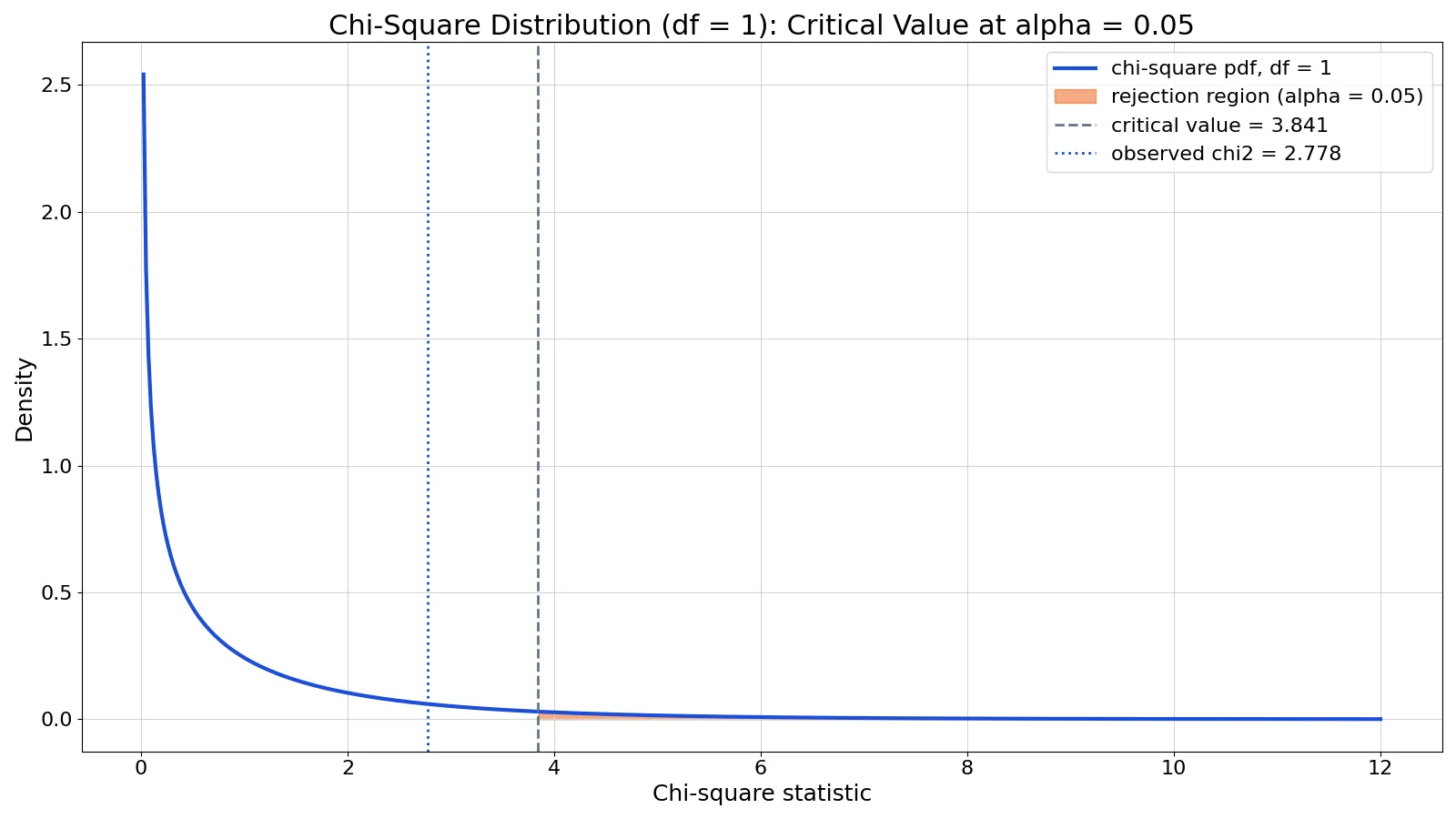
A chi square table lists the cutoff values of the chi-square distribution. You find your critical value by matching your degrees of freedom to a column for your significance level. If your test statistic is larger than that value, you reject the null hypothesis.

Quick Answer

The chi square table is organized by degrees of freedom in the rows and tail probability in the columns.
Most printed tables give upper-tail critical values only, so the column header is the significance level $\alpha$ [1].
For a test of independence or goodness of fit, degrees of freedom come from the table shape, not the sample size.
At $\alpha = 0.05$ and 1 degree of freedom, the critical value is 3.8415.
Reject the null hypothesis when your statistic is greater than the critical value.

Before You Start

You need three things before you open a chi square table.

First, your test statistic. This is the $\chi^2$ value you computed from your observed and expected counts. The formula is

$$\chi^2 = \sum \frac{(O - E)^2}{E}$$

where $O$ is an observed count and $E$ is the expected count under the null hypothesis [2].

Second, your degrees of freedom. For a contingency table with $r$ rows and $c$ columns, the degrees of freedom are

$$df = (r - 1)(c - 1)$$

For a goodness of fit test with $k$ categories, $df = k - 1$ [2].

Third, your significance level $\alpha$. This is the probability of rejecting a true null hypothesis that you are willing to accept, commonly 0.05 or 0.01.

One structural fact matters here. The chi-square distribution is not symmetric, so a single table cannot serve both tails [3]. Most textbook tables give upper-tail values, which is what you need for the standard chi-square test. If you need a lower-tail value, you need a separate table or software [3].

If you want a refresher on what the distribution looks like and why it is skewed, see the chi-square distribution guide.

Step by Step

Compute your test statistic. Sum $(O - E)^2 / E$ across all cells. Keep at least three decimal places.

Find your degrees of freedom. Use $(r-1)(c-1)$ for a contingency table or $k-1$ for goodness of fit. Write it down before you touch the table.

Choose your significance level. Decide on $\alpha$ before you look at the data. Typical choices are 0.10, 0.05, and 0.01.

Locate the row for your degrees of freedom. The leftmost column of the table lists $df$ from 1 upward. Find your exact value.

Locate the column for your significance level. The top row of the table shows $\alpha$ values such as 0.10, 0.05, 0.025, 0.01, and 0.005. Some tables label these columns with $1 - \alpha$ instead, so check the header carefully [3].

Read the value where the row and column meet. That number is your critical value.

Compare. If your test statistic is greater than the critical value, reject the null hypothesis. If it is less than or equal to the critical value, fail to reject [3].

For a two-sided test, the procedure changes. You compare your statistic against the upper-tail value at $1 - \alpha/2$ and the lower-tail value at $\alpha/2$, and you reject if the statistic falls outside that range [3]. Most chi-square tests of independence and goodness of fit are upper-tail only, so you will rarely need this.

Worked Example

A survey collects 100 responses. Each respondent is in group A or group B, and each gives a Yes or No answer. The question is whether the answer depends on the group.

Group	Yes	No	Row total
A	40	20	60
B	20	20	40
Column total	60	40	100

Step 1. Expected counts. Each expected count is row total times column total divided by the grand total.

Group	Yes	No
A	36.0000	24.0000
B	24.0000	16.0000

Step 2. Chi-square statistic. Sum $(O - E)^2 / E$ across the four cells.

$$\chi^2 = \frac{(40-36)^2}{36} + \frac{(20-24)^2}{24} + \frac{(20-24)^2}{24} + \frac{(20-16)^2}{16} = 2.7778$$

Step 3. Degrees of freedom. With 2 rows and 2 columns, $df = (2-1)(2-1) = 1$.

Step 4. Critical value. At $\alpha = 0.05$ and $df = 1$, the table gives 3.8415.

Step 5. Decision. The statistic 2.7778 is less than 3.8415, so you fail to reject the null hypothesis. The p-value is 0.0956, which is above 0.05 and agrees with the table decision.

Here is the same calculation in Python.

from scipy import stats
chi2 = 2.7778
df = 1
crit = stats.chi2.ppf(0.95, df)
p = stats.chi2.sf(chi2, df)
print(chi2, df, crit, p)

2.7778 1 3.841458820694124 0.09557937819379998

The printed critical value rounds to 3.8415 and the p-value rounds to 0.0956, matching the table lookup.

Other Ways to Do It

Printed tables are convenient but limited. You have better options for most work.

Spreadsheet functions. Excel and Google Sheets both provide CHISQ.INV.RT(probability, degrees_freedom), which returns the right-tail critical value. To get 3.8415 for $df = 1$ at $\alpha = 0.05$, pass 0.05 as the probability. The older CHIINV function does the same thing.

Statistical software. In R, qchisq(0.95, df = 1) returns the critical value. In Python, scipy.stats.chi2.ppf(0.95, 1) does the same, as shown above.

Online calculators. A chi-square test calculator takes your observed counts and returns the statistic, degrees of freedom, critical value, and p-value in one step. This avoids the row-and-column lookup entirely.

Interpolation. If your degrees of freedom fall between two rows, you cannot read an exact value from a printed table. Software gives you the exact number. If you must use the table, report the bracketing values instead of a single number.

The same logic applies to other distributions. The critical value table guide covers how cutoff tables work in general, and the F distribution table follows the same row-and-column pattern for ANOVA.

Troubleshooting

Your degrees of freedom are not in the table. Printed tables usually stop at 30, 100, or 200. For larger values, use software. The chi-square distribution approaches a normal distribution as $df$ grows, but the exact value from software is always better.

The column headers look wrong. Some tables label columns with the tail probability $\alpha$, others with $1 - \alpha$. A column headed 0.95 in an upper-tail table means $\alpha = 0.05$ [3]. Read the caption before you read the number.

Your statistic is negative. This is impossible for a chi-square statistic, since every term is a square divided by a positive number. A negative value means an arithmetic error or a mislabeled cell.

You cannot tell whether the test is one-sided or two-sided. Chi-square tests of independence and goodness of fit are upper-tail tests. You reject when the statistic is large. Two-sided versions exist but are uncommon [3].

Your expected counts are small. The chi-square approximation is unreliable when expected counts are below about 5. Combine categories or use an exact test instead.

Common Mistakes

Using the sample size as degrees of freedom. The degrees of freedom come from the table structure, not the number of observations. For a 2x2 table, $df = 1$ no matter how many people you surveyed. Fix: compute $(r-1)(c-1)$ every time.
Reading the wrong column. Confusing $\alpha$ with $1 - \alpha$ shifts your critical value and can flip your decision. Fix: check whether the header says "upper tail area" or "confidence level."
Comparing the p-value to the critical value. These are different quantities. Compare your statistic to the critical value, or compare your p-value to $\alpha$. Do not mix them.
Rejecting when the statistic equals the critical value. The rule is to reject when the statistic is strictly greater [3]. Fix: treat equality as a failure to reject.
Forgetting to check expected counts. A large statistic built on tiny expected counts may be an artifact. Fix: verify that expected counts are at least about 5 before trusting the result.
Using a lower-tail table by accident. The chi-square distribution is asymmetric, so upper and lower tables give different numbers [3]. Fix: confirm which tail your test uses before looking anything up.

Limitations

A chi square table gives you a cutoff, not a conclusion about your research question. It tells you whether the evidence crosses a threshold. It says nothing about effect size, and a large sample can produce a statistically significant result from a trivial association. Report the statistic, the degrees of freedom, and a measure of association strength together.

Printed tables also force you to round. If your degrees of freedom are not listed, you cannot get an exact critical value, and interpolation between rows introduces error. Software removes this problem entirely. The table is a teaching tool and a fallback, not the best available method.

Frequently Asked Questions

What is the difference between a chi square table and a chi square test table?

They are the same thing. Both names refer to a grid of critical values indexed by degrees of freedom and tail probability. Some sources call it a chi square value table or a table for chi square test, and all of these describe the same lookup.

How do I find the critical value for a chi square test?

Compute your degrees of freedom, choose your significance level, then find the row for your degrees of freedom and the column for your significance level. The number where they meet is your critical value. At $\alpha = 0.05$ and $df = 1$, that value is 3.8415.

What if my degrees of freedom are larger than the table goes?

Use software. In Excel, CHISQ.INV.RT(0.05, df) returns the critical value for any degrees of freedom. In R, use qchisq(0.95, df). Printed tables stop at a fixed maximum, but the distribution is defined for any positive degrees of freedom.

Do I reject the null hypothesis if my statistic is smaller than the critical value?

No. You reject when the statistic is greater than the critical value. A smaller statistic means your observed counts are close to what the null hypothesis predicts, so there is not enough evidence against it [3].

Can I use a chi square table for a two-sided test?

Yes, but you need both tails. Compare your statistic against the upper-tail value at $1 - \alpha/2$ and the lower-tail value at $\alpha/2$, and reject if it falls outside that range [3]. Most chi-square tests of independence and goodness of fit are upper-tail only, so this situation is uncommon.

References

6.3: Testing for Goodness of Fit using Chi-Square (Special Topic) - Statistics LibreTexts./06%3A_Inference_for_Categorical_Data/6.03%3A_Testing_for_Goodness_of_Fit_using_Chi-Square_(Special_Topic))
The Chi Squared Test - Statistics LibreTexts
1.3.6.7.4. Critical Values of the Chi-Square Distribution