F Distribution Table: How to Read and Use It

By Dr. Zubair Khalid, DVM, MS, PhD · 2026-10-03

The F distribution table gives you the critical value you compare against an F statistic. You find it by locating the numerator degrees of freedom across the top and the denominator degrees of freedom down the side, then reading the cell where they meet. If your computed F is larger than that value, you reject the null hypothesis at the chosen significance level.

Quick Answer

The F distribution table lists upper-tail critical values of the F distribution, a right-skewed distribution used most often in analysis of variance [1].
Numerator degrees of freedom ($df_1$) label the columns, denominator degrees of freedom ($df_2$) label the rows [1].
Each table is tied to one right-tail probability, usually $\alpha = 0.05$, $0.10$, or $0.01$ [2].
Reject the null hypothesis when your computed F statistic is greater than the tabled critical value [2].
The order of the two degrees of freedom matters. $F(10,12)$ is not the same distribution as $F(12,10)$ [1].

What the F Distribution Table Means

In plain terms, the F distribution table is a lookup grid that tells you how large an F statistic must be before you call it statistically significant. Instead of computing a p-value by hand, you compare your test statistic to a threshold.

The precise definition: the F distribution is the distribution of the ratio of two independent chi-square variables, where each chi-square has first been divided by its degrees of freedom [3]. Its probability density function is

$$f(x) = \frac{\Gamma\left(\frac{\nu_1 + \nu_2}{2}\right) \left(\frac{\nu_1}{\nu_2}\right)^{\frac{\nu_1}{2}} x^{\frac{\nu_1}{2} - 1}}{\Gamma\left(\frac{\nu_1}{2}\right) \Gamma\left(\frac{\nu_2}{2}\right) \left(1 + \frac{\nu_1 x}{\nu_2}\right)^{\frac{\nu_1 + \nu_2}{2}}}$$

where $\Gamma$ is the gamma function [3]. In a testing context the F distribution is treated as a standardized distribution with no location or scale parameters [3]. The cumulative distribution function has no simple closed form, so it is computed numerically [3]. That is exactly why tables exist, and why software is even better.

How It Works

The F statistic is a ratio of two variance estimates:

$$F = \frac{MS_1}{MS_2} = \frac{SS_1 / df_1}{SS_2 / df_2}$$

Each symbol means:

$SS_1$ is the sum of squares for the effect you are testing, such as between-group variation.
$df_1$ is its degrees of freedom, the numerator degrees of freedom.
$SS_2$ is the sum of squares for error or residual variation.
$df_2$ is its degrees of freedom, the denominator degrees of freedom.
$MS_1$ and $MS_2$ are the resulting mean squares.

To read the table, pick the table for your $\alpha$ level. Find your $df_1$ in the column headings and your $df_2$ in the row headings. The cell where they intersect is the critical value. For example, to find the 0.05 critical value for an F distribution with 10 and 12 degrees of freedom, you look in the 10 column and the 12 row of the $\alpha = 0.05$ table, giving $F(0.05, 10, 12) = 2.7534$ [1].

Because the F distribution is asymmetric, a two-sided test needs a different set of tables that cover both the lower and upper rejection regions [2]. Most F tests in ANOVA and regression are one-sided upper-tail tests, so the standard tables are what you need.

Worked Example

The dataset is plant growth in centimeters for 24 plants split across 4 fertilizer groups of 6 plants each.

Fertilizer	Growth (cm)
A	12.1, 13.4, 11.8, 12.9, 13.0, 12.5
B	14.2, 15.1, 14.8, 14.0, 15.3, 14.6
C	13.0, 12.7, 13.5, 12.9, 13.2, 12.8
D	15.5, 16.0, 15.2, 15.8, 15.1, 15.6

The steps:

Grand mean of all 24 measurements: 13.9583.
Group means: A = 12.6167, B = 14.6667, C = 13.0167, D = 15.5333.
Between-group sum of squares: $SSB = \sum n_i(\bar{x}_i - \bar{x})^2 = 34.0150$.
Within-group sum of squares: $SSW = \sum (x - \bar{x}_i)^2 = 4.0833$.
Degrees of freedom: $df_1 = k - 1 = 4 - 1 = 3$ and $df_2 = N - k = 24 - 4 = 20$.
Mean squares: $MSB = 34.0150 / 3 = 11.3383$ and $MSW = 4.0833 / 20 = 0.2042$.
Computed F statistic: $F = 11.3383 / 0.2042 = 55.5347$.
Critical F from the table at $df_1 = 3$, $df_2 = 20$, $\alpha = 0.05$: 3.0984.
Decision: $55.5347 > 3.0984$, so reject $H_0$.
p-value: $1 - F.\text{cdf}(55.5347, 3, 20) = 0.0000$.

Here is the same test in Python.

import numpy as np
from scipy import stats
groups = {'A':[12.1,13.4,11.8,12.9,13.0,12.5],
          'B':[14.2,15.1,14.8,14.0,15.3,14.6],
          'C':[13.0,12.7,13.5,12.9,13.2,12.8],
          'D':[15.5,16.0,15.2,15.8,15.1,15.6]}
arrs = [np.array(v) for v in groups.values()]
F, p = stats.f_oneway(*arrs)
F_crit = stats.f.ppf(1-0.05, 3, 20)
print(F, p, F_crit)  # 55.5347 0.0000 3.0984

Rounded to four decimals, the output is F = 55.5347, p = 0.0000, F_crit(df1=3,df2=20) = 3.0984 (the unrounded p-value is a very small number, not exactly zero). In Excel, =F.INV.RT(0.05,3,20) returns 3.0984. In R, qf(0.95, df1=3, df2=20) returns 3.0984.

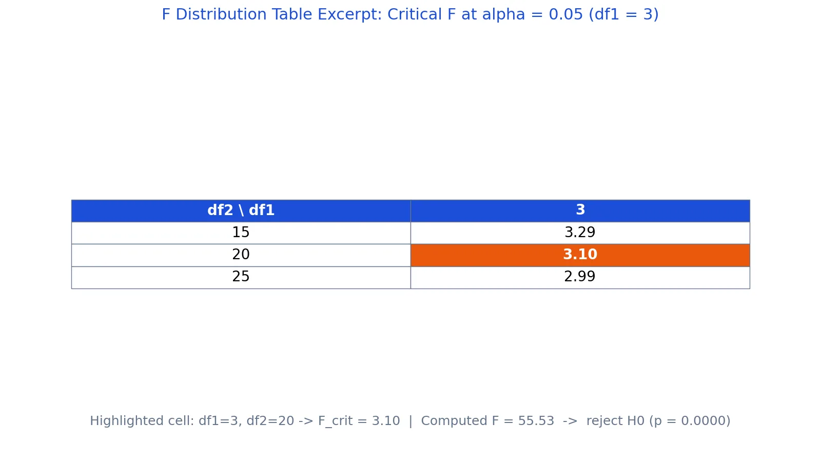
The figure below shows the relevant slice of the table for $df_1 = 3$ at $\alpha = 0.05$: the critical value is 3.29 at $df_2 = 15$, 3.10 at $df_2 = 20$ (highlighted), and 2.99 at $df_2 = 25$. The computed F of 55.53 clears the $df_2 = 20$ threshold by a wide margin.

$df_2$	Critical F ($df_1 = 3$, $\alpha = 0.05$)
15	3.2874
20	3.0984
25	2.9912

How to Interpret It

The critical value splits the F distribution into two zones. Values below it fall in the non-rejection region. Values above it fall in the upper tail, the rejection region at your significance level [2].

Three things drive how large the critical value is:

Smaller $\alpha$ means a larger critical value. The $\alpha = 0.01$ table gives bigger thresholds than the $\alpha = 0.05$ table [2].
More denominator degrees of freedom means a smaller critical value. In the worked example, the threshold drops from 3.2874 at $df_2 = 15$ to 2.9912 at $df_2 = 25$.
The numerator degrees of freedom shift the value too, and the two are not interchangeable [1].

A large F means the variance explained by your model or grouping is large relative to the leftover variance. In the plant example, the fertilizer groups differ far more than the plants within each group do.

When to Use It (and when not to)

Use the F distribution table when you run a one-sided upper-tail F test and want a quick threshold without software. Common cases:

One-way ANOVA comparing means across three or more groups.
Regression overall significance, testing whether the model explains variance beyond chance.
Comparing nested models to see whether added predictors help.
Any variance ratio test where you need a critical value at a set $\alpha$.

Skip the table when you need an exact p-value, when your test is two-sided, or when your degrees of freedom are large enough that software is simply faster. The table only gives thresholds at the $\alpha$ levels it was built for [2]. For a broader look at how thresholds work across distributions, see the critical value table guide.

F Distribution Table vs t Table

Both tables give critical values for a test statistic, but they answer different questions.

Feature	F distribution table	t table
Shape	Right-skewed, starts at 0	Symmetric around 0
Degrees of freedom	Two ($df_1$ and $df_2$)	One
Typical use	ANOVA, regression overall test	Single mean or coefficient test
Tail used	Upper tail for standard tests	One or two tails
Order matters	Yes, $F(10,12) \neq F(12,10)$ [1]	Not applicable

If you are testing one coefficient in a regression, the t table is the right tool. If you are testing the whole model or several group means at once, use the F table. The chi-square table guide covers a related distribution that also uses one tail and one degrees-of-freedom value.

Common Mistakes

Swapping the two degrees of freedom. The numerator value goes in the columns and the denominator in the rows, and switching them changes the answer [1]. Fix: label your $df_1$ and $df_2$ before you open the table.
Using the wrong $\alpha$ table. A value that is significant at 0.05 may not be at 0.01 [2]. Fix: decide your significance level before the test and stick to it.
Reading a two-sided test from a one-sided table. Standard F tables hold only the upper tail [2]. Fix: for a genuinely two-tailed F test, such as comparing two variances, also find the lower-tail critical value. ANOVA and regression F tests stay upper-tail even though their alternatives are non-directional.
Comparing the p-value to the critical value. They are different quantities. Fix: compare your F statistic to the critical value, or compare your p-value to $\alpha$, but do not mix them.
Forgetting that F is always positive. A negative or zero F signals a calculation error. Fix: recheck your sums of squares and mean squares.
Rounding the critical value too early. Small differences matter near the threshold. Fix: keep four decimal places until the final comparison.

Limitations

The table cannot give you an exact p-value. It only tells you whether your statistic crosses a fixed threshold at one of the tabulated $\alpha$ levels [2]. If your F lands just above or just below the critical value, you learn very little about how strong the evidence is. Software that computes the cumulative distribution numerically gives you the full picture [3].

The table also assumes your data meet the F test's conditions, mainly independent observations and normally distributed errors with roughly equal variances. A large F from badly behaved data is not evidence of a real effect. And because the F distribution is asymmetric, one-sided tables cannot serve two-sided tests [2]. When in doubt, compute the exact value.

Frequently Asked Questions

How do I find the critical value in an F distribution table?

Find the table for your significance level, then locate your numerator degrees of freedom in the column headings and your denominator degrees of freedom in the row headings. The cell where the column and row meet is the critical value [1]. For $df_1 = 3$ and $df_2 = 20$ at $\alpha = 0.05$, that value is 3.0984.

Which degrees of freedom go on top?

The numerator degrees of freedom go across the top as column headings, and the denominator degrees of freedom go down the side as row headings [1]. In ANOVA, the numerator is usually the between-group degrees of freedom and the denominator is the within-group or error degrees of freedom.

What does a significant F value mean in ANOVA?

It means the variation between group means is large relative to the variation within groups, so at least one group mean differs from the others. In the plant example, F = 55.5347 against a critical value of 3.0984 gives strong evidence that fertilizer affects growth. The test does not tell you which groups differ, so follow up with pairwise comparisons.

Can I use the F table for regression?

Yes. The overall F test in regression checks whether the model explains a meaningful share of the variance in the outcome. The numerator degrees of freedom equal the number of predictors, and the denominator degrees of freedom equal the residual degrees of freedom. The same table and the same decision rule apply.

Why is the F distribution right-skewed?

It is built as a ratio of two scaled chi-square variables, and a ratio of positive quantities cannot be negative [3]. Most of its probability mass sits near small values, with a long tail stretching to the right. That shape is why the standard tables only cover the upper tail.