ANOVA Table Explained: Components, Formulas and Example

By Dr. Zubair Khalid, DVM, MS, PhD · 2026-10-03

Analysis of variance summarizes a comparison of group means in a single table. ANOVA tables have one row per source of variation and columns for sums of squares, degrees of freedom, mean squares, the F statistic and the p-value. This article explains each cell, shows the formulas, and builds a complete table from raw data.

Quick Answer

An ANOVA table splits total variation into a between-groups part and a within-groups part [1].
Each row reports a sum of squares (SS) and its degrees of freedom (df).
Dividing SS by df gives a mean square (MS), which is a variance estimate [2].
The test statistic is $F = MST / MSE$, the ratio of the two mean squares [2].
A large F with a small p-value suggests at least one group mean differs from the others [3].

What an ANOVA Table Means

An ANOVA table is a standardized summary of an analysis of variance. It lists the sources of variation in your data, the amount of variation each source explains, and the test statistic used to judge whether group means differ.

The precise definition: an ANOVA table partitions the corrected total sum of squares into components that correspond to different sources of variation, then divides each component by its degrees of freedom to form mean squares, and finally forms the ratio of the treatment mean square to the error mean square [1][2]. In a one-way design, the two components are the sum of squares of treatments (between groups) and the sum of squares of error (within groups) [1].

The underlying principle is the law of total variance. Total variance in a dataset breaks down into components attributable to different sources, here the variation between groups and the variation within groups [4].

How It Works

The decomposition for a one-way layout with $k$ groups and $n_i$ observations in group $i$ is:

$$\sum_{i=1}^{k} \sum_{j=1}^{n_i} (y_{ij} - \bar{y}_{\cdot\cdot})^2 = \sum_{i=1}^{k} n_i (\bar{y}_{i\cdot} - \bar{y}_{\cdot\cdot})^2 + \sum_{i=1}^{k} \sum_{j=1}^{n_i} (y_{ij} - \bar{y}_{i\cdot})^2$$

Each symbol:

$y_{ij}$ is observation $j$ in group $i$.
$\bar{y}_{i\cdot}$ is the mean of group $i$.
$\bar{y}_{\cdot\cdot}$ is the grand mean of all observations.
$n_i$ is the number of observations in group $i$.
$N$ is the total number of observations.

The left side is the total sum of squares. The first term on the right is the between-groups sum of squares. The second term is the within-groups sum of squares [1].

Mean squares are formed by dividing each sum of squares by its degrees of freedom [2]. The degrees of freedom for treatments are $k - 1$, and the degrees of freedom for error are $N - k$ [2]. The test statistic is:

$$F = \frac{MST}{MSE}$$

When the null hypothesis of equal means is true, both mean squares estimate the same error variance and their ratio should be close to 1. When the null hypothesis is false, the treatment mean square is inflated and F grows [2]. The critical value comes from the F distribution with $DFT$ and $DFE$ degrees of freedom [2].

A standard one-way table looks like this:

Source	SS	df	MS	F
Between (treatments)	$SSB$	$k-1$	$SSB/(k-1)$	$MSB/MSW$
Within (error)	$SSW$	$N-k$	$SSW/(N-k)$
Total	$SST$	$N-1$

Some authors label the rows "between" and "within" instead of "treatments" and "error" [2].

Worked Example

The dataset below records plant heights in centimeters after four weeks under three fertilizer treatments, with five plants per group.

Fertilizer	Height (cm)
A	12.1
A	13.4
A	11.8
A	12.9
A	13.0
B	15.2
B	14.8
B	15.6
B	15.1
B	14.9
C	10.4
C	11.2
C	10.9
C	11.5
C	10.7

Step 1, the grand mean:

$$(12.1+13.4+11.8+12.9+13.0+15.2+14.8+15.6+15.1+14.9+10.4+11.2+10.9+11.5+10.7) / 15 = 12.9000$$

Step 2, the group means: Fertilizer A is 12.6400, Fertilizer B is 15.1200, Fertilizer C is 10.9400.

Step 3, the between-groups sum of squares. Each group mean is compared with the grand mean, squared, multiplied by the group size, and summed:

$$5(12.6400-12.9000)^2 + 5(15.1200-12.9000)^2 + 5(10.9400-12.9000)^2 = 44.1880$$

Step 4, the within-groups sum of squares, which is the sum of squared deviations of each observation from its own group mean: 2.8920.

Step 5, the total sum of squares: $44.1880 + 2.8920 = 47.0800$.

Step 6, the degrees of freedom. Between: $k - 1 = 3 - 1 = 2$. Within: $N - k = 15 - 3 = 12$. Total: $N - 1 = 15 - 1 = 14$.

Step 7, the mean squares. $MSB = 44.1880 / 2 = 22.0940$. $MSW = 2.8920 / 12 = 0.2410$.

Step 8, the F statistic: $22.0940 / 0.2410 = 91.6763$.

Step 9, the p-value: $P(F(2,12) > 91.6763) = 0.0000$.

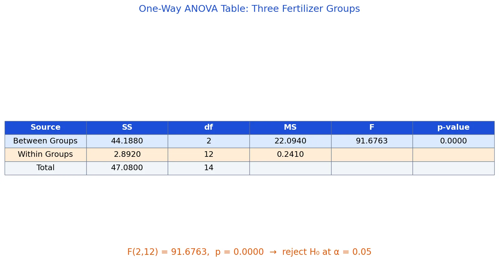
The completed table:

Source	SS	df	MS	F	p
Between	44.1880	2	22.0940	91.6763	0.0000
Within	2.8920	12	0.2410
Total	47.0800	14

You can reproduce this with a few lines of Python:

import numpy as np
from scipy import stats
A = [12.1, 13.4, 11.8, 12.9, 13.0]
B = [15.2, 14.8, 15.6, 15.1, 14.9]
C = [10.4, 11.2, 10.9, 11.5, 10.7]
F, p = stats.f_oneway(A, B, C)
print(f"{F:.4f} {p:.4f}")  # 91.6763 0.0000

Output:

91.6763 0.0000

If you prefer a spreadsheet, the ANOVA Calculator accepts grouped values directly, and the step-by-step guide on how to run ANOVA in Excel covers the built-in tool.

How to Interpret It

Read the table from the bottom row upward. The total row tells you how much variation exists overall. The between row tells you how much of it is explained by group membership. The within row tells you how much remains unexplained.

The F statistic is the comparison that matters. It is the ratio of the between-groups variance estimate to the within-groups variance estimate [2]. A value near 1 means the two estimates agree, which is what you expect when group means are equal. A large value means the between-groups estimate is inflated by real differences among the means [3].

The p-value answers a narrower question: if all group means were truly equal, how often would you see an F at least this large? In the example, F(2,12) = 91.6763 with p = 0.0000, so the observed spread among fertilizer means is very unlikely under equal means. The table does not tell you which fertilizer differs from which. For that you need post-hoc comparisons, such as Tukey, Bonferroni or false discovery rate methods.

The mean square for error is also useful on its own. It is the pooled within-group variance, and its square root is the standard deviation you would use in follow-up calculations.

When to Use It (and when not to)

Use a one-way ANOVA table when you have one categorical factor with three or more levels and one continuous response variable, and you want to test whether the level means differ [5]. It also works for two groups, though a t-test gives the same answer. The comparison of ANOVA and the t-test explains when each is the better fit.

Do not use a one-way table when you have two factors, repeated measurements on the same units, or a response that is a count or a proportion. Two-factor designs need extra rows for the second factor and the interaction, and repeated measurements need a different error structure. The one-way versus two-way comparison covers those differences, and repeated measures versus mixed-effects models covers the longitudinal case.

The test also assumes the response is normally distributed within each group and that within-group variability is similar across groups [5]. Check both before trusting the p-value.

ANOVA Table vs Regression Coefficients

Both approaches model a continuous response, but they report different things.

Aspect	ANOVA table	Regression coefficients
Output	SS, df, MS, F, p per source	Estimate, standard error, t, p per predictor
Question answered	Do any group means differ?	How much does the response change per unit of a predictor?
Categorical predictors	Natural fit, one row per factor	Needs dummy coding
Overall test	F test on the whole model	F test on the whole model
Follow-up	Post-hoc mean comparisons	Individual coefficient tests

The two are connected. Regression is often used to fit a model first, then ANOVA tools are used to test hypotheses about batches of coefficients [4]. If your factor is categorical and your interest is in group means, the ANOVA table is the more direct summary.

Common Mistakes

Reporting only the p-value. The p-value says nothing about effect size. Report the mean squares and the group means so readers can judge practical importance.
Using the total df for the F test. The F ratio uses the between and within degrees of freedom, not the total [2]. In the example that is (2, 12), not (2, 14).
Dividing by the wrong df. Each sum of squares has its own degrees of freedom. Mixing them produces mean squares that do not estimate variances.
Ignoring unequal group sizes. The between-groups formula weights each group mean by its sample size. Treating groups as equal when they are not biases the result.
Skipping the assumptions. Normality within groups and similar within-group variability are required for the F distribution to be the right reference [5].
Running post-hoc tests after a non-significant F. If the overall test does not reject, pairwise comparisons are hard to justify.

Limitations

The table is a summary, not a diagnosis. It cannot tell you which groups differ, whether the difference is meaningful in your field, or whether the design was sound. A significant F only says the between-groups variance is large relative to the within-groups variance [3].

The method is also sensitive to its assumptions. If within-group variances differ substantially, or if the response is strongly skewed, the p-value from the F distribution can be misleading. Outliers inflate the error mean square and can hide real differences, or inflate the between mean square and create differences that are not there. Always look at the raw group data alongside the table.

Frequently Asked Questions

What do the rows of an ANOVA table mean?

Each row is a source of variation. In a one-way design there are three: between groups, within groups and total. The between row captures variation explained by group membership, the within row captures leftover variation, and the total row is their sum [1].

What is the difference between SS and MS?

SS is a sum of squared deviations and depends on the number of observations. MS is that sum divided by its degrees of freedom, which turns it into a variance estimate on a comparable scale [2]. You compare mean squares, not sums of squares.

Why is F a ratio of two mean squares?

Because both mean squares estimate the same error variance when the group means are equal. Their ratio should then be near 1. If group means differ, the between mean square grows and the ratio exceeds 1 [2][3].

Can I get a negative F statistic?

No. Sums of squares are sums of squared quantities, so they cannot be negative, and neither can the mean squares or their ratio. A negative value in your output signals a data entry or coding error.

What sample size do I need for an ANOVA table?

There is no fixed minimum, but each group needs enough observations to estimate its variance. Small groups make the error mean square unstable and reduce power. If you are unsure, run a power calculation before collecting data.