What Is a Confusion Matrix? Definition and Examples

By Dr. Zubair Khalid, DVM, MS, PhD · 2026-10-03

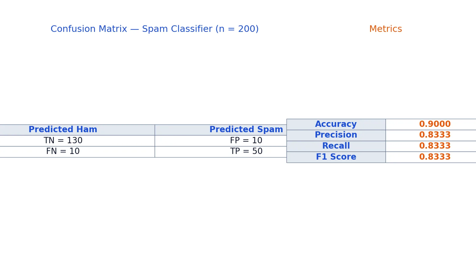
A confusion matrix is a table that counts how a classifier's predictions compare with the true labels. It splits every prediction into one of four cells: true positive, false positive, false negative or true negative. From those four numbers you can read accuracy, precision, recall and F1 without going back to the raw data.

Quick Answer

A confusion matrix is a 2x2 table for binary classification, with actual classes as rows and predicted classes as columns.
The four cells are TP (predicted positive, actually positive), FP (predicted positive, actually negative), FN (predicted negative, actually positive) and TN (predicted negative, actually negative).
Accuracy is the share of all predictions that were correct: $(TP + TN) / \text{total}$.
Precision asks how many predicted positives were right: $TP / (TP + FP)$. Recall asks how many actual positives were found: $TP / (TP + FN)$.
F1 is the harmonic mean of precision and recall, so it stays low if either one is low.

What a Confusion Matrix Means

In plain terms, a confusion matrix is a scorecard that shows where a model gets confused. Instead of reporting one accuracy number, it breaks the errors into two kinds: false alarms and missed cases. That distinction matters because the two errors usually have different costs.

The precise definition: for a binary classifier with a positive class and a negative class, the confusion matrix is the contingency table of predicted labels against actual labels. Each cell holds a count of test observations. The row totals are the actual class sizes and the column totals are the predicted class sizes. Scikit-learn's confusion_matrix function builds this table from y_true and y_pred, and its normalize argument can scale the counts over the true rows, the predicted columns, or the whole population [1]. The older plot_confusion_matrix helper was removed in scikit-learn 1.2 in favor of ConfusionMatrixDisplay.

For more than two classes the same idea extends to an $n \times n$ table. Each row is an actual class and each column is a predicted class, so the diagonal holds correct predictions and the off-diagonal cells hold specific mistakes. The four-cell version below is the binary case.

How It Works

The matrix is filled by comparing each prediction with its true label and incrementing the matching cell. The four counts are:

Cell	Meaning	Predicted	Actual
TP	True positive	Positive	Positive
FP	False positive	Positive	Negative
FN	False negative	Negative	Positive
TN	True negative	Negative	Negative

The four metrics are defined from these counts:

$$\text{Accuracy} = \frac{TP + TN}{TP + FP + FN + TN}$$

$$\text{Precision} = \frac{TP}{TP + FP}$$

$$\text{Recall} = \frac{TP}{TP + FN}$$

$$F1 = \frac{2 \cdot \text{Precision} \cdot \text{Recall}}{\text{Precision} + \text{Recall}}$$

Each symbol is a count. $TP$ is correct positive predictions, $FP$ is negative cases wrongly called positive, $FN$ is positive cases wrongly called negative, and $TN$ is correct negative predictions. Accuracy uses all four because it covers the whole table. Precision ignores $FN$ and $TN$ because it only cares about the predicted-positive column. Recall ignores $FP$ and $TN$ because it only cares about the actual-positive row. F1 combines precision and recall into one number.

Worked Example

Take a spam classifier evaluated on 200 test emails. Of these, 60 are actual spam and 140 are actual ham. The predictions break down like this:

actual	predicted	count
spam	spam	50
spam	ham	10
ham	spam	10
ham	ham	130

Walking through the counts:

Total test rows: 200 = 50 + 10 + 10 + 130
Actual spam (row 1 total): 60 = 50 + 10
Actual ham (row 2 total): 140 = 10 + 130
Predicted spam (column 1 total): 60 = 50 + 10
Predicted ham (column 2 total): 140 = 10 + 130
Accuracy = (TP + TN) / total = (50 + 130) / 200 = 0.9000
Precision = TP / (TP + FP) = 50 / (50 + 10) = 0.8333
Recall = TP / (TP + FN) = 50 / (50 + 10) = 0.8333
F1 = 2 P R / (P + R) = 2 0.8333 0.8333 / (0.8333 + 0.8333) = 0.8333

So TP = 50, FP = 10, FN = 10, TN = 130. Accuracy is 0.9000, precision is 0.8333, recall is 0.8333 and F1 is 0.8333.

You can reproduce this with scikit-learn:

from sklearn.metrics import confusion_matrix, accuracy_score, precision_score, recall_score, f1_score
y_true = [1]*60 + [0]*140
y_pred = [1]*50 + [0]*10 + [1]*10 + [0]*130
print(confusion_matrix(y_true, y_pred))
print(f"{accuracy_score(y_true, y_pred):.4f}")   # 0.9000
print(f"{precision_score(y_true, y_pred):.4f}")  # 0.8333
print(f"{recall_score(y_true, y_pred):.4f}")     # 0.8333
print(f"{f1_score(y_true, y_pred):.4f}")         # 0.8333

Output:

The matrix prints with the negative class first, so the top-left cell is TN = 130 and the bottom-right cell is TP = 50.

How to Interpret It

Read the diagonal first. In the example, 130 ham emails and 50 spam emails were classified correctly. The off-diagonal cells are the errors, and they are not interchangeable. The 10 emails in the spam row predicted as ham are missed spam (false negatives). The 10 ham emails predicted as spam are false alarms (false positives).

Then read the metrics in light of those errors. Accuracy of 0.9000 sounds strong, but it hides the fact that 10 of 60 spam emails slipped through. Precision of 0.8333 means that when the model said "spam," it was right about 83 percent of the time. Recall of 0.8333 means it caught about 83 percent of the actual spam. Because precision and recall are equal here, F1 lands at the same value.

Which metric matters depends on the cost of each error. If a false positive is expensive, watch precision. If a false negative is expensive, watch recall. A study on detecting Parkinson's disease from voice data made this point directly: the highest-accuracy model was not automatically the best one, and the authors argued there may be merit in sacrificing some accuracy to avoid false negatives and favor safer models over more precise ones [2]. The confusion matrix is what exposes that trade-off.

When to Use It (and when not to)

Use a confusion matrix whenever you need to see the shape of a classifier's errors, not just the error rate. It is the standard first diagnostic for binary and multiclass classification, and it is the source of precision, recall and F1. It is also useful when classes are imbalanced, because it shows how many predictions landed in the minority class instead of hiding them inside one aggregate number.

Do not use it as your only evaluation when you need a single ranking score across many models, since a table is harder to sort than a number. Do not use raw counts to compare models trained on test sets of different sizes. If you want to compare across datasets, normalize the matrix over rows, columns or the full population, which is what the normalize argument in scikit-learn's plotting function does [1]. For regression problems, a confusion matrix does not apply because there are no discrete classes to count.

Confusion Matrix vs Contingency Table

The two look alike because both cross-tabulate two categorical variables. The difference is intent and naming.

Aspect	Confusion matrix	General contingency table
Variables	Predicted label vs actual label	Any two categorical variables
Typical use	Evaluating a classifier	Exploring association between variables
Cell names	TP, FP, FN, TN	Generic joint counts
Derived metrics	Accuracy, precision, recall, F1	Chi-square, odds ratios, row percentages
Orientation	Rows are actual, columns are predicted	Either orientation

A confusion matrix is a contingency table with a specific job. If you want to understand how two variables move together in general, a covariance matrix or a contingency table is the better tool.

Common Mistakes

Mixing up rows and columns. Many libraries put actual classes on rows and predicted classes on columns, but some plots flip this. Check the axis labels before reading any cell. Fix: confirm which axis is actual and which is predicted, then label the four cells explicitly.
Assuming accuracy is enough. A model that predicts the majority class every time can score high accuracy while catching zero positives. Fix: always read precision and recall alongside accuracy.
Swapping precision and recall. Precision divides by predicted positives, recall divides by actual positives. Fix: remember that recall measures coverage of the real positives, precision measures trust in the positive predictions.
Comparing raw counts across different test sizes. A matrix with 1,000 rows and one with 100 rows are not directly comparable. Fix: normalize before comparing.
Forgetting which class is "positive." Precision and recall depend entirely on that choice. Fix: state the positive class before reporting any metric.
Reporting F1 without precision and recall. Two very different models can share an F1 value. Fix: report all three so the trade-off is visible.

Limitations

A confusion matrix summarizes predictions at one decision threshold. Change the threshold and the counts change, so the matrix describes a specific operating point, not the model in general. It also gives no information about how confident the model was, only which class it chose. Two models with identical matrices can have very different probability calibration.

For multiclass problems the table grows quickly and becomes hard to read at a glance, and a single aggregate metric can hide which specific class pairs are confused. The matrix also says nothing about why errors happen. It tells you that 10 spam emails were missed, not whether they were short, unusual or mislabeled. Treat it as a starting point for error analysis, not the end of it.

Frequently Asked Questions

What is a confusion matrix in simple terms?

It is a table that counts correct and incorrect predictions for a classifier. Each row is an actual class and each column is a predicted class. The diagonal cells are correct predictions and the off-diagonal cells are the different kinds of mistakes.

What do TP, FP, FN and TN stand for?

TP is a true positive, a positive case correctly predicted positive. FP is a false positive, a negative case wrongly predicted positive. FN is a false negative, a positive case wrongly predicted negative. TN is a true negative, a negative case correctly predicted negative.

How do you calculate accuracy from a confusion matrix?

Add the two correct cells and divide by the total. Accuracy equals $(TP + TN)$ divided by $(TP + FP + FN + TN)$. In the spam example that is $(50 + 130) / 200 = 0.9000$.

When should you use F1 instead of accuracy?

Use F1 when the classes are imbalanced or when both false positives and false negatives matter. Accuracy can look high on imbalanced data even when the minority class is barely detected. F1 balances precision and recall, so it drops when either one is weak.

Can a confusion matrix have more than four cells?

Yes. For $n$ classes it becomes an $n \times n$ table, with one row per actual class and one column per predicted class. The diagonal still holds correct predictions, and each off-diagonal cell shows a specific misclassification between two classes.