What Is a Covariance Matrix? Definition, Formula and Examples

By Dr. Zubair Khalid, DVM, MS, PhD · 2026-10-03

A covariance matrix is a square table that stores the variance of every variable in a dataset along its diagonal and the covariance between every pair of variables in the remaining positions. It summarizes how several numeric variables move together in one compact object. This article defines the covariance matrix, shows the formula for each entry, and walks through a full calculation on real numbers.

Quick Answer

A covariance matrix is a $p \times p$ grid for $p$ variables, where entry $(i, j)$ is the covariance between variable $i$ and variable $j$.
The diagonal entries are variances, so $C[i, i]$ is the variance of variable $i$ alone.
The off-diagonal entries are covariances, so $C[i, j]$ measures how variables $i$ and $j$ move together.
The matrix is symmetric, meaning $C[i, j] = C[j, i]$, because covariance has no direction.
A positive off-diagonal value means the two variables tend to rise and fall together, a negative value means one tends to rise as the other falls.

What a Covariance Matrix Means

In plain terms, a covariance matrix is a summary table for a group of numeric variables. Instead of reporting one variance per variable and one covariance per pair, you stack them all into a single square matrix. The National Institute of Standards and Technology describes it as a matrix with "the variances along the main diagonal and the covariances between each pair of variables in the other matrix positions" [1].

The precise statistical definition is this. Suppose you have $n$ observations and $p$ variables, and let $X_i$ be the $p \times 1$ column vector of values for observation $i$. The sample covariance matrix is

$$ S = \frac{1}{n-1} \sum_{i=1}^n (X_i - \bar{X})(X_i - \bar{X})' $$

where $\bar{X}$ is the mean vector. Each diagonal entry of $S$ is a variance and each off-diagonal entry is a covariance [1]. The same object is also called the variance-covariance matrix or the dispersion matrix [1].

How It Works

Every entry in the matrix comes from one formula. For two variables $X$ and $Y$ measured on the same $n$ observations, the sample covariance is

$$ \text{COV}(X, Y) = \frac{\sum_{i=1}^{n}(X_i - \bar{x})(Y_i - \bar{y})}{n-1} $$

Here is what each symbol means.

$X_i$ and $Y_i$ are the values of the two variables for observation $i$.
$\bar{x}$ and $\bar{y}$ are the arithmetic means of $X$ and $Y$.
$n$ is the number of observations.
$n - 1$ in the denominator gives the unbiased sample estimate, matching the usual sample variance [1].

When $X$ and $Y$ are the same variable, the formula collapses to the variance, which is why the diagonal holds variances. The full matrix for variables $X$, $Y$, and $Z$ looks like this.

$$ C = \begin{bmatrix} \text{Var}(X) & \text{Cov}(X,Y) & \text{Cov}(X,Z) \\ \text{Cov}(Y,X) & \text{Var}(Y) & \text{Cov}(Y,Z) \\ \text{Cov}(Z,X) & \text{Cov}(Z,Y) & \text{Var}(Z) \end{bmatrix} $$

Because $\text{Cov}(X,Y) = \text{Cov}(Y,X)$, the matrix is symmetric across its diagonal. If you want to see how a single pair is computed before building the full grid, the covariance formula walkthrough covers that step by step.

Worked Example

The dataset below records 20 students' weekly study hours, nightly sleep hours, and exam score.

study_hours	sleep_hours	exam_score
2.5	8.5	52
3.0	8.0	55
3.5	7.5	58
4.0	7.0	62
4.5	7.5	65
5.0	6.5	68
5.5	7.0	70
6.0	6.0	73
6.5	6.5	75
7.0	6.0	78
7.5	5.5	80
8.0	6.0	83
8.5	5.5	85
9.0	5.0	88
9.5	5.5	90
10.0	5.0	92
10.5	4.5	94
11.0	5.0	96
11.5	4.5	98
12.0	4.0	100

The number of students is $n = 20$. The mean study hours are 7.2500 and the mean exam score is 78.1000.

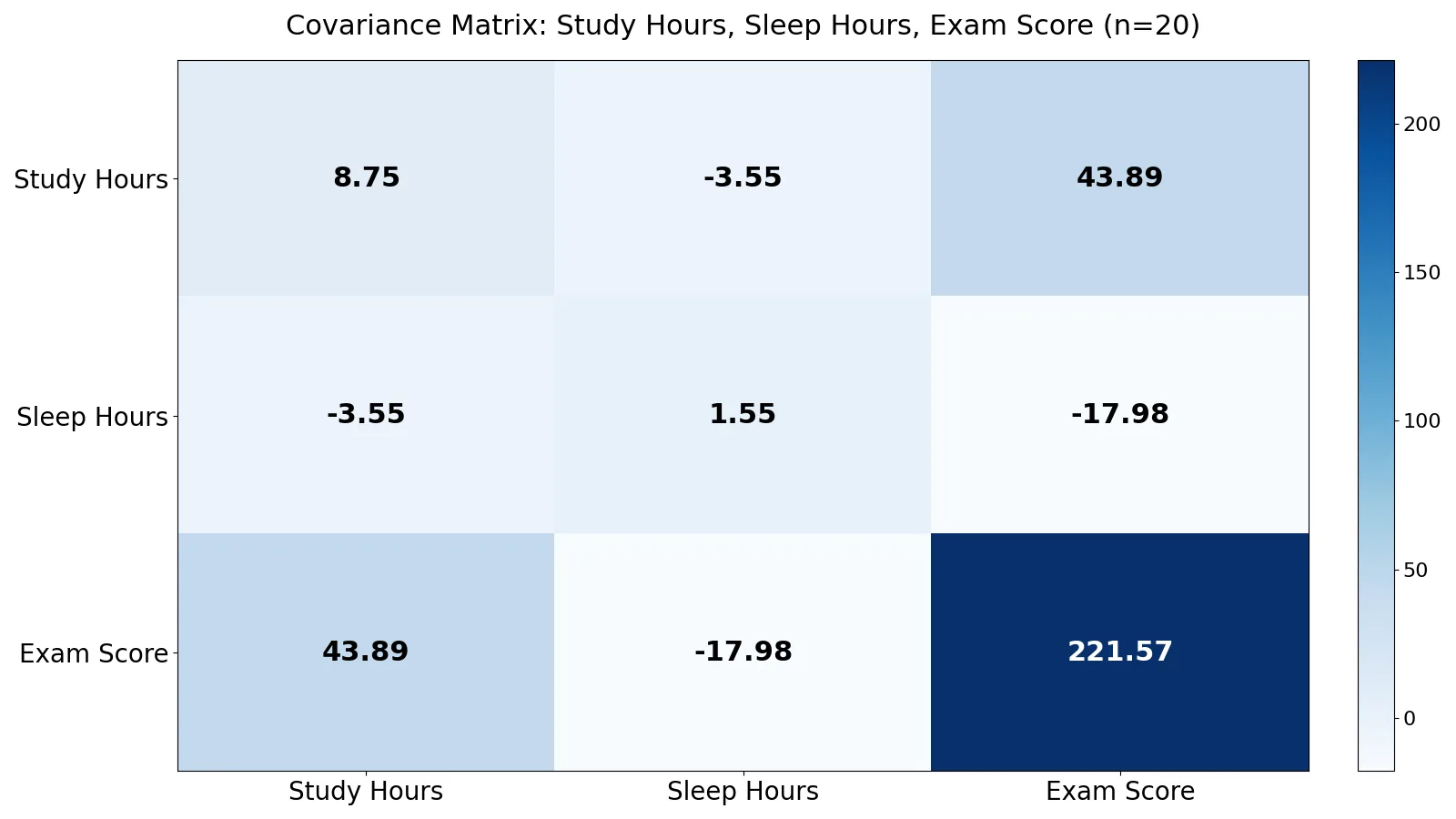
The diagonal entries are variances. The variance of study hours is $\sum (x_i - 7.2500)^2 / (n-1) = 8.7500$. The variance of sleep hours is 1.5500. The variance of exam score is 221.5684.

The off-diagonal entries are covariances. The covariance between study hours and exam score is $\sum (x_i - 7.2500)(y_i - 78.1000) / (n-1) = 43.8947$. The covariance between study hours and sleep hours is -3.5526. The covariance between sleep hours and exam score is -17.9789.

Assembling these values gives the full matrix.

$$ C = \begin{bmatrix} 8.7500 & -3.5526 & 43.8947 \\ -3.5526 & 1.5500 & -17.9789 \\ 43.8947 & -17.9789 & 221.5684 \end{bmatrix} $$

You can reproduce this in Python with NumPy.

import numpy as np
data = np.array([
    [2.5, 8.5, 52], [3.0, 8.0, 55], [3.5, 7.5, 58], [4.0, 7.0, 62],
    [4.5, 7.5, 65], [5.0, 6.5, 68], [5.5, 7.0, 70], [6.0, 6.0, 73],
    [6.5, 6.5, 75], [7.0, 6.0, 78], [7.5, 5.5, 80], [8.0, 6.0, 83],
    [8.5, 5.5, 85], [9.0, 5.0, 88], [9.5, 5.5, 90], [10.0, 5.0, 92],
    [10.5, 4.5, 94], [11.0, 5.0, 96], [11.5, 4.5, 98], [12.0, 4.0, 100],
])
cov = np.cov(data, rowvar=False, ddof=1)
print(cov)

Output:

[[8.7500 -3.5526 43.8947]
 [-3.5526 1.5500 -17.9789]
 [43.8947 -17.9789 221.5684]]

How to Interpret It

Read the diagonal first. Each diagonal value is the spread of one variable on its own. Exam score has the largest variance at 221.5684, so scores vary widely across students. Sleep hours have the smallest variance at 1.5500, so sleep is fairly consistent.

Then read the off-diagonal values for direction and strength. The covariance between study hours and exam score is 43.8947, a positive number, so students who study more tend to score higher. The covariance between study hours and sleep hours is -3.5526, so students who study more tend to sleep less. The covariance between sleep hours and exam score is -17.9789, so more sleep goes with lower scores in this dataset.

The sign tells you direction, but the size is hard to judge because it depends on the units. Study hours are measured in hours and exam score in points, so 43.8947 mixes those units. To compare relationships on a common scale, divide the covariance by the product of the two standard deviations to get a correlation. For study hours and exam score that gives $43.8947 / (\sqrt{8.7500} \times \sqrt{221.5684}) = 0.9969$. For study hours and sleep hours it gives -0.9647, and for sleep hours and exam score it gives -0.9702. The correlation vs covariance comparison explains why the standardized version is often easier to report.

When to Use It (and when not to)

Use a covariance matrix when you work with several numeric variables at once and want one object that captures all their spreads and pairwise relationships. It is the natural input for multivariate methods such as principal component analysis, where the eigenvectors of the covariance matrix define the directions of greatest variation, and for the multivariate normal distribution, which takes a covariance matrix as a shape parameter [2]. It also appears in portfolio risk, where the diagonal holds each asset's variance and the off-diagonal entries hold how pairs of assets move together.

Do not use it as a standalone measure of relationship strength. Covariance values are unit-dependent, so a large covariance can reflect large units instead of a strong relationship. If you need to compare relationships across different pairs of variables, use a correlation matrix. Also avoid it when your variables are on wildly different scales and you have not standardized them, because the largest-variance variable will dominate any downstream analysis.

Covariance Matrix vs Correlation Matrix

The two matrices have the same shape and the same symmetry, but they answer slightly different questions. A covariance matrix keeps the original units. A correlation matrix rescales each pair to a value between -1 and 1.

Feature	Covariance matrix	Correlation matrix
Diagonal values	Variances of each variable	All 1s
Off-diagonal values	Covariances in original units	Correlations between -1 and 1
Units	Depends on the variables	Unitless
Sensitive to scale	Yes	No
Typical use	PCA, multivariate normal, portfolio risk	Comparing relationship strength

Common Mistakes

Reading a large covariance as a strong relationship. The fix is to standardize by dividing by the product of standard deviations and report the correlation instead.
Confusing the diagonal with covariances. The fix is to remember that the diagonal always holds variances, one per variable.
Using $n$ instead of $n - 1$ in the denominator. The fix is to use $n - 1$ for the unbiased sample estimate, as in the formula above [1].
Forgetting that the matrix is symmetric. The fix is to compute only the upper triangle and mirror it, since $C[i, j] = C[j, i]$.
Comparing covariances across pairs with different units. The fix is to move to a correlation matrix before ranking relationships.
Ignoring missing values. The fix is to decide how missing data are handled, since different software defaults can change which observations enter each pair [3].

Limitations

A covariance matrix only captures linear relationships. If two variables follow a strong curved pattern, their covariance can be near zero even though they are clearly related. It also says nothing about causation, only about how variables move together in the observed data.

The matrix is sensitive to outliers, because a single extreme observation can shift both a variance and several covariances at once. It also grows quickly with the number of variables. With $p$ variables you store $p(p+1)/2$ unique values, so wide datasets produce large matrices that are hard to read directly. In practice, analysts often work with a decomposition of the matrix instead of the full grid, since many calculations are more efficient that way [2].

Frequently Asked Questions

What is the difference between a covariance matrix and a variance-covariance matrix?

They are the same object under two names. The term variance-covariance matrix emphasizes that the diagonal holds variances and the off-diagonal holds covariances, while covariance matrix is the shorter common form [1].

Why is the covariance matrix symmetric?

Because covariance does not depend on order. The covariance between $X$ and $Y$ equals the covariance between $Y$ and $X$, so entry $(i, j)$ always equals entry $(j, i)$ and the matrix mirrors across its diagonal.

Can a covariance matrix have negative values?

Yes. Off-diagonal entries can be negative, which means the two variables tend to move in opposite directions. In the worked example, the covariance between study hours and sleep hours is -3.5526. Diagonal entries cannot be negative because a variance is never below zero.

How do I turn a covariance matrix into a correlation matrix?

Divide each covariance by the product of the two corresponding standard deviations. The standard deviations are the square roots of the diagonal entries. This rescales every off-diagonal value to a correlation between -1 and 1 while the diagonal becomes all 1s.

What does a covariance matrix tell me about my data?

It tells you how much each variable varies on its own and how each pair of variables moves together. The signs of the off-diagonal entries show direction, and the diagonal entries show spread. For strength comparisons across pairs, convert it to a correlation matrix first.