Python for Machine Learning: A Beginner's Guide

By Dr. Zubair Khalid, DVM, MS, PhD · 2026-10-03

Python machine learning means using the Python language and its scientific libraries to build models that learn patterns from data. You load a dataset, split it into training and test parts, fit a model, then measure how well it predicts. This guide walks through that workflow with a small worked example you can run yourself.

Quick Answer

Python is the most common language for machine learning because its libraries cover the whole workflow, from arrays to model training to evaluation [1].
NumPy provides the array structure that most other libraries build on, and SciPy adds scientific algorithms on top of it [1][2].
scikit-learn gives you ready-made models such as support vector machines and neural networks with a consistent fit and predict interface [3][4].
A basic workflow is: load data, split into train and test, standardize features, fit a model, predict, then score.
Accuracy alone can mislead. A confusion matrix shows which classes the model confuses.

What Python Machine Learning Means

In plain terms, Python machine learning is the practice of writing Python code that lets a computer find patterns in data and use those patterns to make predictions. You do not hand-code the rules. You show the model examples and it adjusts itself.

The precise definition: machine learning is the process of estimating a function $f$ that maps input features $X$ to a target $y$, by minimizing a loss function over a set of training examples. In Python, that estimation is done by numerical libraries that operate on arrays of numbers. NumPy is the primary array programming library for Python and the foundation the scientific Python ecosystem is built on [1]. SciPy extends it with scientific algorithms and has become a standard for that kind of computing in Python [2].

How It Works

The mechanism has three moving parts: data as arrays, a model with parameters, and a loss function that measures error.

For a classification problem, a common model is multinomial logistic regression. It turns a score for each class into a probability:

$$P(y=k \mid x) = \frac{\exp(w_k \cdot x)}{\sum_j \exp(w_j \cdot x)}$$

$x$ is the feature vector for one sample.
$w_k$ is the weight vector for class $k$.
$w_k \cdot x$ is the dot product, a single score for class $k$.
The denominator sums those exponentiated scores over all classes $j$, so the outputs are probabilities that add to 1.

Training means finding the weights $w_k$ that make the correct class most likely across all training rows. That is done by gradient descent, which repeatedly nudges the weights in the direction that lowers the loss. The loss for this model is cross-entropy, the negative log of the probability assigned to the true class.

scikit-learn wraps this in a consistent interface. Every estimator has a fit method that takes arrays X and y, and a predict method that returns predicted labels [4]. Support vector machines follow the same pattern and use a subset of training points, called support vectors, in the decision function [3].

Worked Example

We use a simplified iris dataset with 15 rows, two features (sepal length and petal length) and three species.

sepal_length_cm	petal_length_cm	species
5.1	1.4	setosa
4.9	1.4	setosa
4.7	1.3	setosa
5.0	1.5	setosa
5.4	1.7	setosa
7.0	4.7	versicolor
6.4	4.5	versicolor
6.9	4.9	versicolor
5.5	4.0	versicolor
6.5	4.6	versicolor
6.3	6.0	virginica
5.8	5.1	virginica
7.1	5.9	virginica
6.3	5.6	virginica
6.5	5.8	virginica

The steps and their computed values:

Dataset size: n = 15 rows, features = 2, classes = 3.
Train/test split: train n = 9, test n = 6, stratified and deterministic.
Feature standardization: sepal mean = 6.0222, sd = 0.8829. Petal mean = 3.9111, sd = 1.8592.
Model: softmax over class scores, $P(y=k \mid x) = \exp(w_k \cdot x) / \sum_j \exp(w_j \cdot x)$.
Gradient descent: 2000 iterations, learning rate 0.1, final loss = 0.2823.
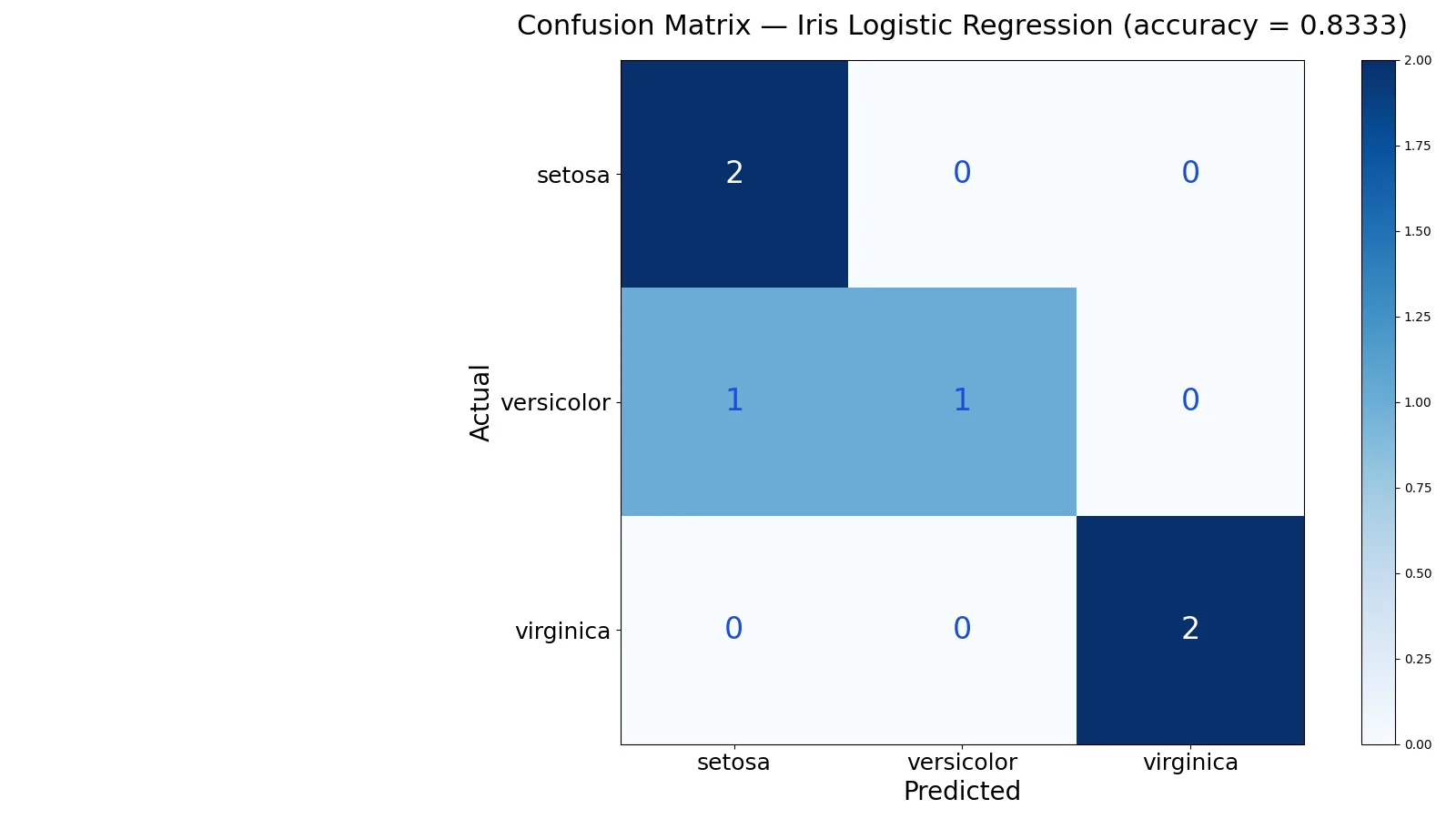
Accuracy: correct = 5 / 6 = 0.8333.

The scikit-learn code below runs the same workflow on the full 150-row iris dataset. With a 30-row test set it prints an accuracy of 1.0, so its numbers differ from the 15-row example. The output shown after the code is from the 15-row example.

from sklearn.datasets import load_iris
from sklearn.linear_model import LogisticRegression
from sklearn.model_selection import train_test_split
from sklearn.metrics import accuracy_score, confusion_matrix
X, y = load_iris(return_X_y=True)
Xtr, Xte, ytr, yte = train_test_split(X, y, test_size=0.2, random_state=0)
clf = LogisticRegression(max_iter=2000).fit(Xtr, ytr)
pred = clf.predict(Xte)
print(accuracy_score(yte, pred))  # 1.0 on the full dataset
print(confusion_matrix(yte, pred))

Output of the 15-row example:

accuracy = 0.8333
confusion_matrix =
[[2 0 0]
 [1 1 0]
 [0 0 2]]

The confusion matrix has rows for the true class and columns for the predicted class, in the order setosa, versicolor, virginica. Setosa is classified perfectly (2 of 2). Versicolor loses one row to setosa (1 of 2). Virginica is perfect (2 of 2). Accuracy is 5 correct out of 6, which is 0.8333.

How to Interpret It

Accuracy tells you the share of test rows the model got right. Here that is 0.8333, or about 83 percent. On a test set of only 6 rows, one mistake moves the number by roughly 17 percentage points, so treat it as a rough signal, not a precise score.

The confusion matrix is more informative than the single number. It shows where errors land. In this run, the model confuses one versicolor flower with setosa, which suggests those two classes are harder to separate with only sepal and petal length. If you want to understand why a model separates classes the way it does, the geometry behind support vector machines is a useful next step.

Always compare accuracy against a baseline. Predicting the most common class every time gives a reference point. If your model cannot beat that, it has learned nothing useful.

When to Use It (and when not to)

Use Python machine learning when you have labeled examples, a clear target, and enough rows to train and test on. It fits classification, regression, clustering and dimensionality reduction tasks, and the same workflow applies across all of them. If you are exploring a new dataset, start with dataset examples and types to understand what you are working with.

Do not reach for machine learning when a simple rule or a spreadsheet formula answers the question. Do not use it when you have very few rows, since models will memorize them. Do not use it when the data has leakage, meaning information from the test set sneaks into training. And do not use it when you cannot explain the result to the people who will act on it.

Python Machine Learning vs Traditional Statistical Modeling

Both fit a model to data. They differ in emphasis, not in kind.

Aspect	Python machine learning	Traditional statistical modeling
Main goal	Prediction accuracy	Explanation and inference
Typical output	Predicted labels or values	Coefficients with standard errors
Model choice	Often chosen by validation score	Often chosen by theory
Data size	Handles large datasets well	Often used on smaller samples
Evaluation	Accuracy, confusion matrix, error metrics	p-values, confidence intervals

If you care about why a variable matters, statistical modeling is usually the better fit. If you care about how well you can predict a new case, machine learning is usually the better fit. For a deeper treatment of the statistical side, see Introduction to Statistical Learning.

Common Mistakes

Skipping the train/test split. If you score on the same rows you trained on, the result is inflated. Fix: hold out a test set before you fit anything.
Forgetting to standardize features. Models that use distances or gradients are sensitive to scale. Fix: standardize on the training set, then apply the same means and standard deviations to the test set.
Tuning on the test set. Every time you check the test score and adjust, you leak information. Fix: use a validation split or cross-validation for tuning, and touch the test set once.
Reporting accuracy on imbalanced data. A model that predicts the majority class can look accurate while being useless. Fix: report a confusion matrix and per-class metrics.
Ignoring the random seed. Results shift between runs. Fix: set random_state so your numbers are reproducible.
Assuming more features help. Extra features can add noise and slow training. Fix: start with a small feature set and add only what improves validation performance.

Limitations

Python machine learning cannot tell you whether your data is representative. A model trained on a biased sample will produce biased predictions, and the accuracy score will not reveal that. It also cannot establish causation. A model that predicts well may rely on a feature that happens to correlate with the target in your sample.

The workflow itself has limits. Results depend on the split, the seed, the hyperparameters and the preprocessing choices, so a single accuracy number is fragile. On small test sets, as in the example above, one row can swing the score by a large margin. Treat any single number as one measurement, not a verdict.

Frequently Asked Questions

What Python libraries do I need for machine learning?

Start with NumPy for arrays, pandas for tabular data, and scikit-learn for models and evaluation. NumPy is the foundation the rest of the scientific Python stack is built on [1]. SciPy adds scientific algorithms when you need them [2]. Add a plotting library when you want to visualize results.

Do I need to know math to do Python machine learning?

You need comfort with basic algebra and the idea of a function. Understanding means, standard deviations and probability helps you interpret results. You do not need to derive the optimization by hand to use scikit-learn, but knowing what gradient descent does makes debugging much easier.

How much data do I need to train a model?

It depends on the problem and the number of features. More features usually require more rows. A practical approach is to start with what you have, use cross-validation, and watch whether validation scores stabilize as you add data. If they swing wildly, you need more rows.

Why is my accuracy different every time I run the code?

Random processes in the split and in model initialization change the result. Setting random_state in the split and in the model makes runs reproducible. If you still see variation, you may be comparing different data or different preprocessing steps.

Can I use Python machine learning without scikit-learn?

Yes. You can implement models directly with NumPy arrays, and SciPy provides optimization routines you can call [2]. Building a model by hand is a good way to learn the mechanics. For real projects, scikit-learn saves time and reduces bugs.

If you want to go further, clustering with K-Means and classification with Naive Bayes are natural next topics, and multivariate analysis covers the broader picture of working with several variables at once.

References

- Harris CR, Millman KJ, van der Walt SJ et al. (2020). Array programming with NumPy. Nature
- Virtanen P, Gommers R, Oliphant TE et al. (2020). SciPy 1.0: fundamental algorithms for scientific computing in Python. Nature Methods
- 1.4. Support Vector Machines, scikit-learn 1.9.1 documentation
- 1.17. Neural network models (supervised), scikit-learn 1.9.1 documentation
Further Reading
- 1.12. Multiclass and multioutput algorithms, scikit-learn 1.9.1 documentation
- Lever J, Krzywinski M, Altman N (2016). Classification evaluation. Nature Methods
Related Articles
- K-Nearest Neighbors (KNN): Algorithm and Examples
- Bayesian Classifiers: How Naive Bayes Works
- Support Vector Machines (SVM): Definition and Examples
- What Is Random Forest? Algorithm and Examples
- K-Means Clustering: How It Works With a Worked Example
- Introduction To Statistical Learning
- How to Learn Machine Learning for Computational Biology
- Elements Of Statistical Learning