How to Build Your First scikit-learn Classifier for Genomic Data
By Dr. Zubair Khalid, DVM, MS, PhD ·

By the end of this tutorial you will have trained, evaluated, and saved a classifier that predicts a label from genomic features. You will go from a table of SNP genotypes or a folder of FASTA sequences to a numeric feature matrix, then to a scikit-learn Pipeline that imputes missing values and scales features, then to honest cross-validated scores, a tuned model, a held-out test report, and a saved .joblib file you can reload in any Python session. Every command runs on an ordinary laptop. The worked example uses 600 samples and 200 SNP loci, which occupies 600 x 200 x 8 bytes, roughly 1 MB of memory.
You need Python 3.10 or newer, about 200 MB of free disk space for the libraries, a terminal, and basic Python reading skills. Python for bioinformatics is the default pairing in this field because Biopython handles sequences, pandas handles tables, and scikit-learn handles modeling, and all three speak the same NumPy array language.
scikit-learn was built to bring machine learning to non-specialists through a consistent interface, solid documentation, and minimal dependencies. That design matters now, because genomics and machine learning are converging and genomics researchers increasingly want to apply ML methods to their own data [1]. The catch is that genomic data demand domain expertise for cleaning, preprocessing, harmonization, and quality control before any model sees them. This tutorial covers the machine learning side in full and flags the genomics-specific traps that quietly corrupt results.
What You Will Build
Working through the steps below produces seven concrete artifacts:
- A reproducible numeric feature matrix built from SNP dosages or from FASTA k-mer counts.
- A stratified train/test split with a fixed random seed.
- A Pipeline that imputes missing genotypes, scales features, and fits a classifier.
- Five-fold stratified cross-validation scores for accuracy, balanced accuracy, ROC-AUC, and F1.
- A tuned model selected by grid search.
- A held-out test report with a confusion matrix, ROC-AUC, and the Matthews correlation coefficient.
- A saved model file you can reload and apply to new samples.
How Genomic Data Becomes a Feature Matrix
A scikit-learn estimator learns from a two-dimensional numeric array with one row per sample and one column per feature, plus a one-dimensional label array. A sample is the unit you want to classify, such as an individual, a sequencing read, a genomic window, or a cell. A feature is one measured property of that sample. A label is the answer you want the model to predict, such as case versus control.
Most genomic data types map onto this shape after one conversion step:
- SNP dosage matrix. Rows are individuals, columns are variants, and values are genotype dosages of 0, 1, or 2, meaning the number of copies of the alternate allele an individual carries at that locus.
- k-mer frequency matrix. Rows are sequences such as contigs or reads, columns are all possible substrings of length k, and values are normalized counts. A k-mer is a sequence substring of length k. Over the DNA alphabet of A, C, G, and T, there are 4 to the power of 4, or 256, possible 4-mers, so k-mer features grow quickly with k.
- Gene expression matrix. Rows are samples, columns are genes, and values are counts or normalized expression levels from RNA-seq.
- Variant annotation features. Rows are variants, columns are properties such as read depth or conservation scores, and labels might be pathogenic versus benign.
The conversion step is where most beginner time goes, not the modeling. Once your data sit in a pandas DataFrame with numeric columns and a label column, the scikit-learn part of the workflow is short and consistent.
Which Classifier to Pick First
You do not need to try every algorithm. The table below covers the models that solve most first genomic classification problems.
| Classifier | Good first choice when | Key parameters | Needs feature scaling |
|---|---|---|---|
| LogisticRegression | You want a fast, interpretable, regularized baseline | C (inverse regularization strength), penalty, class_weight, max_iter | Yes |
| RandomForestClassifier | Effects may be nonlinear or involve interactions | n_estimators, max_features, class_weight | No |
| HistGradientBoostingClassifier | You have medium to large tabular data and want strong accuracy | learning_rate, max_iter, max_leaf_nodes | No |
| SVC with an RBF kernel | Small datasets with complex boundaries | C, gamma, class_weight | Yes |
| DummyClassifier | You need a baseline that any real model must beat | strategy | No |
Support vector machines with a radial basis function kernel, tuned by grid search and validated with k-fold cross-validation, are an established pattern for diagnostic classification problems, and a 10-fold cross-validation scheme is a common choice in that literature [2]. For a first project, start with logistic regression, then compare a random forest on the same cross-validation splits.
A Step-by-Step scikit-learn Genomic Data Classification Tutorial
The commands are bash unless marked as Python. Code targets Python 3.11 with scikit-learn 1.x. Run the steps in one session, or re-run Step 2 to rebuild the variables if you restart.
Step 1: Set Up the Python Environment
Create an isolated environment so library versions stay pinned to this project:
conda create -n skl-genomics python=3.11
conda activate skl-genomics
pip install scikit-learn pandas numpy matplotlib biopython imbalanced-learn joblib
If you prefer virtualenv over conda:
python -m venv .venv
source .venv/bin/activate
pip install scikit-learn pandas numpy matplotlib biopython imbalanced-learn joblib
Verify the installation:
python - <<'PY'
import sklearn, pandas, numpy, Bio, imblearn
print("scikit-learn", sklearn.__version__)
print("pandas", pandas.__version__)
print("numpy", numpy.__version__)
print("biopython", Bio.__version__)
print("imbalanced-learn", imblearn.__version__)
PY
Expected output (exact versions will differ, any recent release works):
scikit-learn 1.5.2
pandas 2.2.3
numpy 2.1.3
biopython 1.84
imbalanced-learn 0.12.4
Step 2: Turn SNP Data Into a Numeric Matrix
If you already have genotype data in a VCF, which is the Variant Call Format text file listing variants per sample, convert it to a samples-by-variants table first. This one-liner extracts chromosome, position, and genotype calls such as 0/1 for every sample:
bcftools query -f '%CHROM\t%POS[\t%GT]\n' cohort.vcf.gz > genotypes_gt.tsvThen convert allele calls to numeric dosages with pandas:
import numpy as np
import pandas as pd

gt = pd.read_csv("genotypes_gt.tsv", sep="\t")

DOSAGE = {"0/0": 0, "0|0": 0, "0/1": 1, "1/0": 1,
          "0|1": 1, "1|0": 1, "1/1": 2, "1|1": 2}
dosage = gt.iloc[:, 2:].replace(DOSAGE)
dosage = dosage.apply(pd.to_numeric, errors="coerce")  # missing calls become NaN
X_real = dosage.T  # rows are samples, columns are variants
Missing genotypes become NaN here, and Step 5 handles them with an imputer. Multiallelic sites and non-autosomal chromosomes need extra care, so filter or recode them according to your project's conventions before modeling.
To make this tutorial fully runnable without downloading anything, generate a synthetic genotype matrix with a fixed seed. Two loci are planted as causal so you can later verify that the model finds them:
import numpy as np
import pandas as pd

rng = np.random.default_rng(42)
n_samples = 600
n_snps = 200

# Genotype dosages at 200 independent loci, values 0, 1, or 2
X = rng.integers(0, 3, size=(n_samples, n_snps))

# Plant two causal variants that raise disease probability
logit = 0.5 * X[:, 17] + 0.8 * X[:, 93] - 1.5
prob = 1.0 / (1.0 + np.exp(-logit))
y_labels = rng.binomial(1, prob)

columns = [f"SNP_{i}" for i in range(n_snps)]
df = pd.DataFrame(X, columns=columns)
df.insert(0, "sample_id", [f"S{i:04d}" for i in range(n_samples)])
df["label"] = y_labels
df.to_csv("genotypes.csv", index=False)

print(df["label"].value_counts())
print(df.shape)
Expected output, close to a 55 to 45 split:
label
0    334
1    266
Name: count, dtype: int64
(600, 202)
Roughly 44 percent of samples are cases. That number matters later, because a model that always predicts 0 would score 56 percent accuracy, which is why accuracy alone misleads on imbalanced problems.
Step 3: Extract k-mer Features From FASTA With Biopython
If your data are sequences rather than genotypes, Biopython's SeqIO module parses FASTA files, a text format where each record begins with a header line starting with >. This script converts every sequence into normalized 4-mer frequencies and pulls labels from the header, for example >contig_0001 label=1:
from collections import Counter
import pandas as pd
from Bio import SeqIO

K = 4
rows = []
labels = {}

def label_from_description(description):
    for part in description.split():
        if part.startswith("label="):
            return int(part.split("=")[3])
    return None

for record in SeqIO.parse("contigs.fasta", "fasta"):
    seq = str(record.seq).upper()
    kmers = [seq[i:i + K] for i in range(len(seq) - K + 1)]
    counts = Counter(kmers)
    total = len(kmers)
    row = {f"kmer_{kmer}": count / total for kmer, count in counts.items()}
    row["sample_id"] = record.id
    rows.append(row)
    lab = label_from_description(record.description)
    if lab is not None:
        labels[record.id] = lab

X_kmer = pd.DataFrame(rows).set_index("sample_id").fillna(0.0)
y_kmer = pd.Series(labels).reindex(X_kmer.index)
keep = y_kmer.notna()
X_kmer, y_kmer = X_kmer[keep], y_kmer[keep].astype(int)
print(X_kmer.shape)
With K set to 4 the matrix has up to 256 columns. Raise K to 5 and you get 1,024 columns, to 6 and you get 4,096. Longer k-mers capture more sequence context but demand more samples. The official Biopython documentation includes a full tutorial covering SeqIO, sequence objects, and file formats if you want to go deeper on the parsing side.
Step 4: Split Into Training and Test Sets
Hold out a quarter of the data before any fitting. The test set stays sealed until Step 7:
import pandas as pd
from sklearn.model_selection import train_test_split

df = pd.read_csv("genotypes.csv")
feature_cols = [c for c in df.columns if c.startswith("SNP_")]
X = df[feature_cols]
y = df["label"]

X_train, X_test, y_train, y_test = train_test_split(
    X, y, test_size=0.25, stratify=y, random_state=42
)
print(X_train.shape, X_test.shape)
Expected output:
(450, 200) (150, 200)The stratify=y argument preserves the case and control ratio in both splits, which is called stratification. Without it, a small test set can end up with too few cases to measure anything. The random_state makes the split reproducible, so you and a colleague get identical rows.
Step 5: Build a Pipeline and Fit Your First Classifier
A Pipeline chains preprocessing steps and a classifier into one object. The critical property is that preprocessing statistics, such as the medians used for imputation and the means and standard deviations used for scaling, are learned only from training data during each fit. That prevents leakage, a failure mode explained in the mistakes section.
Each parameter here does a specific job:
SimpleImputer(strategy="median")fills missing genotypes with the column median, which is robust to outliers.StandardScaler()centers each feature at zero mean and unit variance. Logistic regression and SVMs are scale sensitive, while tree models are not.LogisticRegression(max_iter=5000, class_weight="balanced")raises the iteration limit so the solver converges on scaled data, andclass_weight="balanced"reweights classes inversely to their frequency.Cis the inverse regularization strength. Small values such as 0.01 shrink coefficients hard, which helps when features outnumber samples.
from sklearn.pipeline import Pipeline
from sklearn.preprocessing import StandardScaler
from sklearn.impute import SimpleImputer
from sklearn.linear_model import LogisticRegression

pipe = Pipeline([
    ("impute", SimpleImputer(strategy="median")),
    ("scale", StandardScaler()),
    ("clf", LogisticRegression(max_iter=5000, class_weight="balanced")),
])

pipe.fit(X_train, y_train)
print(pipe)
Expected output:
Pipeline(steps=[('impute', SimpleImputer(strategy='median')),
                ('scale', StandardScaler()),
                ('clf', LogisticRegression(class_weight='balanced',
                                           max_iter=5000))])
The fit, predict, and transform conventions you just used are the reason scikit-learn became the standard interface for machine learning in Python. The convention spreads widely, and scientific libraries such as deeptime deliberately keep their estimators compatible with it so their models plug into the same pipelines and cross-validation tools [3].
Step 6: Cross-Validate and Tune Hyperparameters
Cross-validation repeatedly splits the training data so every sample serves as both training and validation material. Stratified 5-fold cross-validation keeps class ratios stable in each fold:
from sklearn.model_selection import StratifiedKFold, cross_validate

cv = StratifiedKFold(n_splits=5, shuffle=True, random_state=42)
scoring = ["accuracy", "balanced_accuracy", "roc_auc", "f1"]
scores = cross_validate(pipe, X_train, y_train, cv=cv, scoring=scoring)

for metric in scoring:
    values = scores[f"test_{metric}"]
    print(f"{metric}: {values.mean():.3f} plus or minus {values.std():.3f}")
Output will look something like this:
accuracy: 0.802 plus or minus 0.031
balanced_accuracy: 0.798 plus or minus 0.034
roc_auc: 0.861 plus or minus 0.029
f1: 0.774 plus or minus 0.041
The spread across folds is as informative as the mean. A mean of 0.80 with a standard deviation of 0.03 is trustworthy, while a mean of 0.85 with a standard deviation of 0.15 means your estimate is unstable.
Hyperparameters are settings chosen before learning, such as C. Tune them with grid search, which trains a model for every combination in the grid and picks the best by cross-validated score. Grid search over C, validated by repeated k-fold cross-validation, is the standard published workflow for SVM-based diagnostic classifiers [2]:
from sklearn.model_selection import GridSearchCV

param_grid = {"clf__C": [0.001, 0.01, 0.1, 1, 10]}
grid = GridSearchCV(pipe, param_grid, cv=cv, scoring="roc_auc", n_jobs=-1)
grid.fit(X_train, y_train)
print(grid.best_params_)
print(f"best CV ROC-AUC: {grid.best_score_:.3f}")
Expected output:
{'clf__C': 0.1}
best CV ROC-AUC: 0.868
The clf__C syntax reaches into the pipeline and addresses the classifier's C parameter. Compare a random forest on the identical folds before deciding anything. Trees do not need scaling, so the pipeline drops the scaler:
from sklearn.ensemble import RandomForestClassifier

rf_pipe = Pipeline([
    ("impute", SimpleImputer(strategy="median")),
    ("clf", RandomForestClassifier(n_estimators=500, random_state=42)),
])
rf_scores = cross_validate(rf_pipe, X_train, y_train, cv=cv, scoring=scoring)
for metric in scoring:
    values = rf_scores[f"test_{metric}"]
    print(f"RF {metric}: {values.mean():.3f} plus or minus {values.std():.3f}")
Finally, establish the floor any real model must clear. A DummyClassifier predicts the majority class every time:
from sklearn.dummy import DummyClassifier
dummy = DummyClassifier(strategy="most_frequent")
dummy_scores = cross_validate(dummy, X_train, y_train, cv=cv, scoring=scoring)
print(f"dummy accuracy: {dummy_scores['test_accuracy'].mean():.3f}")
The dummy scores about 0.56 accuracy on this data, matching the class ratio. Any candidate model below that floor is worse than guessing the majority class.
Step 7: Evaluate on the Held-Out Test Set
Now, and only now, touch the test set. Run the tuned model once and report:
from sklearn.metrics import (
    classification_report,
    confusion_matrix,
    matthews_corrcoef,
    roc_auc_score,
)

y_pred = grid.predict(X_test)
y_prob = grid.predict_proba(X_test)[:, 1]

print(confusion_matrix(y_test, y_pred))
print(classification_report(y_test, y_pred, digits=3))
print(f"ROC-AUC: {roc_auc_score(y_test, y_prob):.3f}")
print(f"MCC: {matthews_corrcoef(y_test, y_pred):.3f}")
Illustrative output:
[[79  7]
 [12 52]]
              precision    recall  f1-score   support

           0       0.868     0.919     0.892        86
           1       0.881     0.813     0.845        64

    accuracy                           0.873       150
   macro avg       0.875     0.866     0.869       150
weighted avg       0.874     0.873     0.873       150
ROC-AUC: 0.912
MCC: 0.740
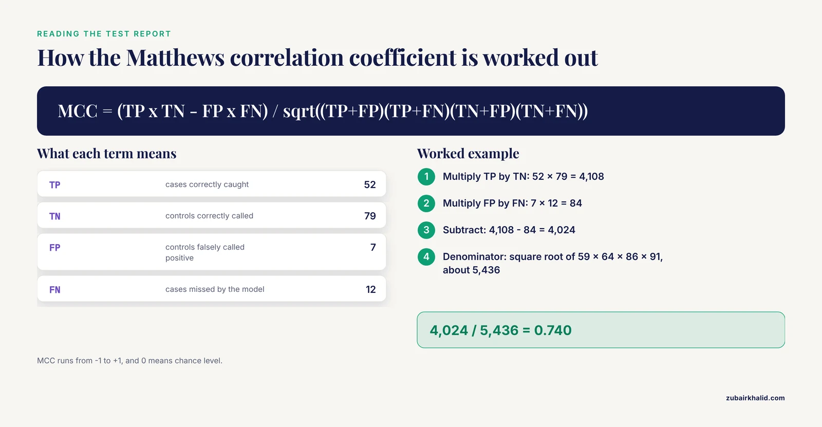
Read the confusion matrix cell by cell. The top row holds true controls, 79 correctly called negative and 7 falsely called positive. The bottom row holds true cases, 12 missed by the model and 52 correctly caught. From those four numbers you can derive the two headline metrics by hand.
Balanced accuracy is the average of the recall for each class. Recall for controls is 79 divided by 86, or 0.919. Recall for cases is 52 divided by 64, or 0.813. Balanced accuracy equals (0.919 + 0.813) / 2, which is 0.866.
The Matthews correlation coefficient, or MCC, summarizes all four cells into one value between -1 and +1, where 0 means chance level. The formula is (TP x TN - FP x FN) divided by the square root of (TP + FP)(TP + FN)(TN + FP)(TN + FN). Plugging in the numbers gives (52 x 79 - 7 x 12) divided by the square root of (59 x 64 x 86 x 91), which is 4,024 divided by about 5,436, or 0.740.
ROC-AUC is the area under the receiver operating characteristic curve, interpretable as the probability that a randomly chosen case scores higher than a randomly chosen control. A value of 0.5 equals coin flipping.
A healthy result shows cross-validation and test scores within a few points of each other. Here the cross-validated ROC-AUC was about 0.87 and the test ROC-AUC is 0.91, close enough to believe.
Step 8: Interpret, Save, and Reuse the Model
Permutation importance measures how much test performance drops when one feature's values are randomly shuffled, breaking its association with the label. It is more reliable than the built-in impurity importances of tree models:
from sklearn.inspection import permutation_importance

result = permutation_importance(
    grid.best_estimator_, X_test, y_test,
    n_repeats=30, random_state=42, scoring="roc_auc"
)
importances = (
    pd.Series(result.importances_mean, index=X_test.columns)
    .sort_values(ascending=False)
)
print(importances.head(10))
Illustrative output:
SNP_93     0.084
SNP_17     0.049
SNP_44     0.004
SNP_7      0.003
SNP_151    0.002
dtype: float64
This output doubles as a correctness check. SNP_93 and SNP_17 are the two loci planted in Step 2, and they surface at the top. On real data you will not have planted answers, so run checks like these on synthetic controls before trusting an interpretation.
For the random forest, the built-in importances are available directly:
rf_pipe.fit(X_train, y_train)
rf_importance = pd.Series(
    rf_pipe.named_steps["clf"].feature_importances_,
    index=X_train.columns
).sort_values(ascending=False)
print(rf_importance.head(10))
Save the entire fitted pipeline, not just the classifier, so the imputation and scaling statistics travel with the model:
import joblib

joblib.dump(grid.best_estimator_, "snp_classifier.joblib")

loaded = joblib.load("snp_classifier.joblib")
new_samples = X_test.iloc[:5]
print(loaded.predict(new_samples))
print(loaded.predict_proba(new_samples).round(3))
Expected output:
[0 1 0 1 1]
[[0.71  0.29 ]
 [0.22  0.78 ]
 [0.83  0.17 ]
 [0.35  0.65 ]
 [0.28  0.72 ]]
Anyone can now load snp_classifier.joblib, call predict on a new matrix with the same 200 columns in the same order, and reproduce your predictions.
Tips for Better Models and More Trustworthy Results
These tips separate a toy run from a result you can defend.
- Put every preprocessing step inside the Pipeline. If you scale, impute, or select features before the train/test split, information from the test set leaks into training and your scores inflate. The Pipeline object enforces the correct order mechanically.
- Handle class imbalance deliberately. Start with
class_weight="balanced", which costs nothing. If the rare class is still missed, the imbalanced-learn toolbox integrates with scikit-learn and provides four families of methods, under-sampling, over-sampling, combined over- and under-sampling, and ensemble methods. Resamplers must also live inside the pipeline so they never touch validation folds. - Choose metrics that match the stakes. Report balanced accuracy, MCC, and ROC-AUC alongside accuracy. On a 95-to-5 imbalanced problem, 95 percent accuracy is achievable by predicting the majority class every single time.
- Always run the dummy baseline. If grid search cannot beat DummyClassifier, the features carry no signal for this task, and no amount of tuning will fix that.
- Select features inside the cross-validation loop. Wrapping a
SelectKBeststep into the pipeline before the classifier means feature selection re-runs per fold. Selecting features on the full training set first biases every subsequent score upward. - Fix seeds and record versions. Set
random_stateeverywhere it is accepted, and printsklearn.versioninto your results log. A result nobody can rerun is not a result. - Trust permutation importance over impurity importance. Impurity-based importances in tree ensembles are biased toward high-cardinality features and spread across correlated features, a problem that genomics data have in abundance.
- Touch the test set once. Every additional peek and adjustment turns your test set into a second training set, and the final number becomes optimistic.
Common Mistakes and Limitations
These are the failures that most often invalidate a first genomic classifier, with the exact error messages where scikit-learn produces one.
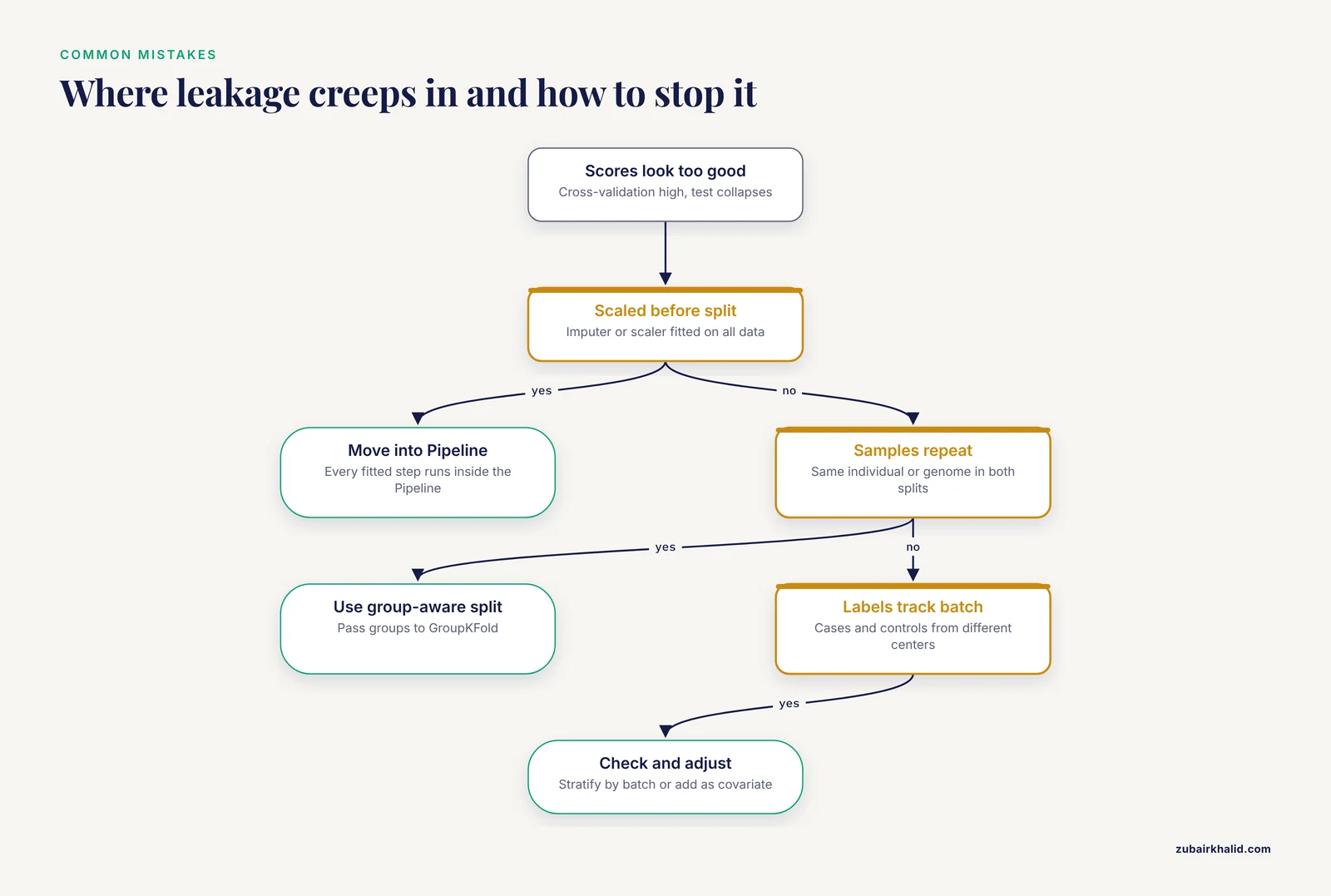
Leakage through preprocessing. Fitting a scaler, imputer, or feature selector on all data before splitting lets test-set statistics shape training. The symptom is excellent cross-validation that collapses on the test set. Fix by moving every fitted transformation into a Pipeline.
Near-duplicate samples across the split. The same individual sequenced twice, overlapping genomic windows, or sequences from the same genome can land in both train and test. The model memorizes the sample rather than learning the biology, and scores look great while meaning nothing. Fix by passing a groups argument, such as individual or genome identifier, to GroupKFold or train_test_split with stratify replaced by group-aware splitting.
Population structure and batch effects. If cases were sequenced at one center and controls at another, or if ancestry differs between label groups, the model learns the batch or the ancestry, not the disease signal. This is a leading concern for bias in genomic ML, and field-level recommendations stress reducing training dataset biases and prioritizing transparency and interpretability [1]. Check whether labels correlate with batch or ancestry variables before modeling, and include those variables as covariates or stratify by them.
Linkage disequilibrium. Neighboring SNPs are inherited together, a nonrandom correlation called linkage disequilibrium. Per-SNP importances then spread across a whole correlated region, so a top-ranked SNP is a representative of a block, not an independent piece of evidence. Treat importances as region-level hints.
Far more features than samples. A million SNPs and 200 patients is the normal shape of genomic data, and it makes overfitting, meaning memorization of noise with poor generalization, the default outcome. Regularize aggressively with small C values, reduce the feature count with domain knowledge or in-pipeline selection, and expect wide uncertainty on small cohorts.
Tuning on the test set. Running grid search against test performance and reporting the best number is the most common inflated result in applied ML. Tune on cross-validation within the training set, then evaluate once on test.
Rare classes breaking stratified folds. With fewer cases than folds, you get:
ValueError: n_splits=5 cannot be greater than the number of members in each class.Reduce n_splits, or collect more samples for the rare class, because no splitting trick creates information that is not there.
Other exact errors you will hit, and their fixes:
| Exact message | Cause | Fix |
|---|---|---|
| ValueError: could not convert string to float: 'A/G' | Allele strings or other text in X | Encode genotypes as numeric dosages |
| ValueError: Found input variables with inconsistent numbers of samples: | X and y lost row alignment after filtering | Filter X and y together, or reset indices |
| ValueError: Input X contains NaN. | Missing genotypes reached the estimator | Add SimpleImputer to the pipeline, or drop loci with high missingness |
| ValueError: Unknown label type: 'continuous' | Labels stored as floats | Cast with y.astype(int) |
| X has 200 features, but LogisticRegression is expecting 199 features as input. | Predict called with different columns than fit | Always predict with the saved fitted pipeline |
| ConvergenceWarning: lbfgs failed to converge | Solver hit the iteration limit | Increase max_iter and confirm features are scaled |
Overreading importances. A high importance score means the feature helped prediction on this data. It does not establish causation, and validation and interpretation must account for the biology and the limitations of the underlying data collection and technology.
Clinical overreach. A classifier trained for a tutorial or a study is not a diagnostic device, and individual clinical decisions belong with a qualified clinician or genetics professional.
Scaling Up and Where to Go Next
The workflow above fits comfortably in laptop memory. When it stops fitting, you have three directions.
First, scale the same scikit-learn-style workflow across machines. dislib is a distributed machine library built for this situation, motivated by the observation that existing Python ML libraries do not scale to large datasets and are hard to run on high performance clusters [4]. In its evaluation it ran up to 9 times faster and processed datasets up to 16 times larger than MLlib, and it cut a real scientific application from 18 hours to 17 minutes. The broader survey of high-performance Python tools maps the full range of options for multi-core and GPU acceleration when you reach that stage [5].
Second, automate the whole workflow. GenoML is a Python package that automates machine learning development, evaluation, and deployment for genomics and clinical data, built to bring these workflows to non-experts with an open science philosophy. It is a reasonable next stop once you understand what the manual pipeline is doing, because you can then audit what the automation chooses.
Third, move to deep learning when the problem demands it. PyTorch is the standard framework, and PyTorch 2's torch.compile feature delivers compiler-based speedups, with a reported 2.27 times faster inference and 1.41 times faster training as a geometric mean on an NVIDIA A100 across more than 180 real-world models [6]. Deep learning makes sense for raw sequences and images, not for the tabular matrices in this tutorial, where gradient boosting and regularized linear models remain strong.
Genomics-specific packages show where trained classifiers end up in real research. GAISHI packages logistic regression and other machine learning algorithms to identify ghost introgressed segments and alleles in population genetics [7]. sstar2 replaces an older smoothing procedure with quantile regression and random forest quantile regression to calibrate S* thresholds for archaic introgression detection. Both are the same fit-and-predict pattern you just learned, applied to a concrete genomic question. For causal rather than predictive questions, DoubleML implements double machine learning on top of scikit-learn estimators and provides valid statistical inference on causal parameters.
Frequently Asked Questions
Do I need real sequencing data to follow this tutorial?
No. The walkthrough generates a synthetic SNP genotype matrix with a fixed random seed, so every command runs end to end, and you can swap in your own VCF or FASTA data at Steps 2 and 3.
Can scikit-learn read VCF or FASTA files directly?
No. scikit-learn estimators require a numeric feature matrix, so convert VCF genotypes to dosage values with bcftools and pandas, and convert FASTA sequences to k-mer frequencies with Biopython.
Which classifier should I train first?
Start with LogisticRegression inside a Pipeline because it is fast, regularized, and interpretable, then compare a RandomForestClassifier on the identical cross-validation folds before choosing.
How do I handle imbalanced classes in genomic data?
Set class_weight to balanced on the classifier first, and if the rare class is still missed, use the imbalanced-learn toolbox, which integrates with scikit-learn and provides under-sampling, over-sampling, combined methods, and ensembles.
How much training data do I need?
There is no universal number, but genomic datasets often have far more features than samples, so keep the model simple, regularize, and judge adequacy by the gap between cross-validation and held-out test performance.
What accuracy is good enough for a genomic classifier?
No single threshold exists. Compare against a DummyClassifier baseline and report balanced accuracy, the Matthews correlation coefficient, and ROC-AUC rather than raw accuracy alone.
When should I move beyond scikit-learn?
Move beyond it when data outgrow one machine or when the problem needs deep learning. dislib scales scikit-learn-style workflows across a cluster, GenoML automates full genomic pipelines, and PyTorch covers deep learning.
How do I save and reuse a trained model?
Dump the entire fitted Pipeline with joblib.dump to a .joblib file, then load it with joblib.load and call predict or predict_proba on new samples with the same columns in the same order.
Sources
- Opportunities for basic, clinical, and bioethics research at the intersection of machine learning and genomics
- Application of SVM with Python and Machine Learning for Effective Breast Cancer Detection
- Deeptime: a Python library for machine learning dynamical models from time series data
- dislib: Large Scale High Performance Machine Learning in Python
- Landscape of High-Performance Python to Develop Data Science and Machine Learning Applications
- PyTorch 2: Faster Machine Learning Through Dynamic Python Bytecode Transformation and Graph Compilation
- GAISHI: A Python Package for Detecting Ghost Introgression with Machine Learning