What Is Random Forest? Algorithm and Examples

By Dr. Zubair Khalid, DVM, MS, PhD · 2026-10-03

A random forest is an ensemble machine learning method that trains many decision trees and combines their predictions into one answer. Each tree sees a different random sample of the rows and a random subset of the features at every split, so the trees make different mistakes. Averaging or voting across them cancels much of that error, which is why a random forest usually beats a single decision tree on new data.

Quick Answer

A random forest builds hundreds of decision trees, each on a bootstrap sample of the data, and combines their outputs by majority vote (classification) or averaging (regression) [1].
Two sources of randomness drive the method: bagging (random rows) and feature sampling (random columns at each split) [2].
The randomness decorrelates the trees, which corrects the overfitting habit of individual decision trees [1][3].
You can estimate accuracy for free with out-of-bag (OOB) predictions, using the rows each tree never saw.
Feature importances tell you which variables drove the splits, but they are not causal effects.

What Random Forest Means

In plain terms, a random forest is a committee of decision trees. You ask hundreds of slightly different trees the same question and let them vote. No single tree is trusted, and the group answer is steadier than any one member.

The precise statistical definition: random forests are an ensemble learning method for classification, regression and other tasks that works by creating a multitude of decision trees during training. For classification, the output is the class selected by most trees. For regression, the output is the average of the tree predictions [1]. The method was formalized by Leo Breiman in 2001 [4].

The name comes from the two random ingredients. "Forest" refers to the collection of trees. "Random" refers to the random row samples and random feature subsets used to grow them [2].

How It Works

The algorithm repeats four steps for each tree in the forest.

Step 1: Draw a bootstrap sample. From your $n$ rows, draw $n$ rows with replacement. Some rows appear several times, others not at all. The rows left out are "out-of-bag" for that tree.

Step 2: Grow the tree with feature randomness. At each split, consider only a random subset of $m$ features instead of all of them. A common default for classification is $m = \sqrt{p}$, where $p$ is the number of features [2].

Step 3: Grow deep, do not prune. Each tree is grown to the largest extent possible, with no pruning [5].

Step 4: Aggregate. For classification, take the majority vote. For regression, take the mean prediction [1].

Two quantities control the forest error rate: the correlation between any two trees, and the strength of each individual tree. Higher correlation raises the error rate, and stronger individual trees lower it. The parameter $m$ trades one against the other, and the OOB error rate helps you find a good value quickly [5].

The Gini impurity at a node measures how mixed the classes are:

$$G = 1 - \sum_{k=1}^{K} p_k^2$$

Here $K$ is the number of classes, and $p_k$ is the proportion of samples at that node belonging to class $k$. A pure node has $G = 0$. Splits are chosen to reduce this value, and summing those reductions across the forest produces the Gini feature importances [2].

Worked Example

The dataset is an Iris-like flower table: 60 rows, 4 numeric features (sepal_len, sepal_wid, petal_len, petal_wid) and 3 species with 20 rows each. Here are the first few rows.

sepal_len	sepal_wid	petal_len	petal_wid	species
5.1738	3.8397	1.6477	0.1521	setosa
4.9516	3.3323	1.5343	0.1814	setosa
5.2267	3.4203	1.4769	0.0894	setosa
5.5331	2.9726	1.4398	0.0804	setosa
4.9180	3.2367	1.2043	0.2813	setosa
5.8011	2.3754	4.5769	1.3455	versicolor
6.0607	2.6738	3.9817	1.5614	versicolor
6.1127	3.1877	5.7431	2.5787	virginica
6.9935	2.7429	5.8243	1.5332	virginica
7.1793	2.6787	6.0332	2.1716	virginica

Walking through the settings and results:

Dataset size: $n = 60$ rows, 4 features, 3 classes.
Bootstrap samples per tree: 60 rows drawn with replacement.
Features tried per split: $m = \sqrt{4} = 2$.
Number of trees: $B = 200$.
Gini impurity at the root: $G = 1 - \sum p_k^2 = 0.6667$, since each class holds one third of the rows.
OOB predictions collected: all 60 rows received at least one OOB vote.
OOB accuracy: 58 correct out of 60, or 0.9667.
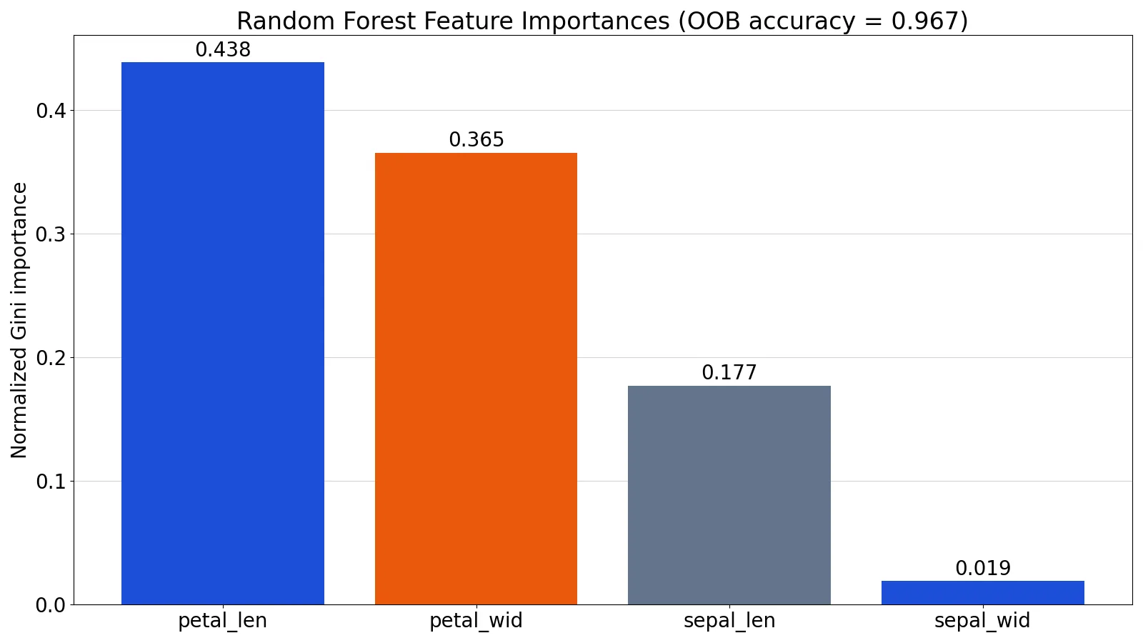
Feature importances (normalized): sepal_len = 0.1772, sepal_wid = 0.0190, petal_len = 0.4384, petal_wid = 0.3655.

The code that produced these numbers:

from sklearn.ensemble import RandomForestClassifier
clf = RandomForestClassifier(n_estimators=200, oob_score=True, random_state=42)
clf.fit(X, y)

Output: OOB accuracy = 0.9667, top feature = petal_len (0.4384).

The bar chart of normalized Gini importances shows petal_len highest at 0.438, with OOB accuracy 0.967. Petal length and petal width together account for about 0.80 of the total importance, while sepal width contributes almost nothing at 0.019.

How to Interpret It

Read three outputs from a fitted forest.

OOB accuracy. Each tree predicts only the rows it did not see during training. Comparing those predictions to the true labels gives an accuracy estimate without a separate validation split. In the example, 58 of 60 rows were classified correctly.

Feature importances. These are normalized to sum to 1. Gini importance, also called mean decrease in impurity (MDI), measures the total reduction in Gini impurity from all splits on a variable, averaged over the trees. Permutation importance, also called mean decrease accuracy (MDA), measures the average accuracy drop when you randomly shuffle a feature's values in the OOB samples [2]. When features are correlated, MDI can spread credit unevenly, so permutation importance on held-out data is often the safer read [4].

Prediction confidence. The share of trees voting for the winning class is a rough confidence score. A 190-to-10 split is a stronger signal than a 105-to-95 split.

A high training accuracy in a random forest is normal and does not mean the model is overfitted [3]. Judge the model on OOB or test accuracy instead.

When to Use It (and when not to)

Use a random forest when you have tabular data with mixed numeric and categorical features, when you want strong accuracy with little tuning, when you need feature importances, or when nonlinear relationships and interactions make a linear model a poor fit. It handles large datasets and many features well [2].

Skip it when you need a model you can explain to a non-technical audience as a single rule set. A single decision tree is easier to draw and defend. Skip it when inference on individual coefficients matters, since a forest gives you importances but not signed effects. Skip it when training speed or memory is tight, because the algorithm is slow to process data since it computes results for each individual tree, and it needs more resources to store that data [2]. For very large tabular problems, gradient boosting is a strong alternative [6].

Random Forest vs Decision Tree

Aspect	Single decision tree	Random forest
Splits considered	All features at each split [2]	Random subset of features [2]
Training data per tree	Full dataset	Bootstrap sample of rows
Overfitting	Prone to overfit the training set [1]	Corrects that habit through averaging [1]
Pruning	Often pruned for control	Trees grown fully, no pruning [5]
Accuracy	Lower and unstable	Usually higher and steadier [5]
Interpretability	One readable flowchart	Many trees, read via importances
Speed and memory	Fast, light	Slower, heavier [2]

Common Mistakes

Judging the model on training accuracy. A forest can reach near 100% on training data and still generalize well [3]. Fix: report OOB or test accuracy.
Treating Gini importances as causal effects. A high importance means the feature helped split the data, not that changing it changes the outcome. Fix: confirm with permutation importance on held-out data [2].
Ignoring correlated features. MDI splits credit between correlated variables and can understate both. Fix: check correlation and use permutation importance [4].
Leaving the number of trees too low. Fewer trees means a noisier vote. Fix: raise the tree count and watch where OOB error flattens.
Forgetting to set a random seed. Results shift between runs. Fix: set random_state for reproducible output [4].
Assuming the default feature count is optimal. The value of $m$ is the one parameter the method is somewhat sensitive to [5]. Fix: tune it against OOB error.

Limitations

A random forest cannot tell you the direction or size of a feature's effect. Importances are non-negative and sum to 1, so a variable that matters in opposite directions in different regions can look unimportant. Correlated predictors make the ranking unstable, and MDI computed on training data is biased toward features with many possible split points [4].

The method is also expensive. Training hundreds of deep trees takes more time and memory than a single tree, and prediction requires running every tree [2]. Extrapolation is another weak spot. Because predictions are averages of tree outputs, a forest cannot predict outside the range of the training targets in regression. It also gives no p-values, no confidence intervals and no closed-form equation you can hand to a colleague.

Frequently Asked Questions

What is random forest in simple terms?

It is a group of decision trees that vote on the answer. Each tree trains on a random sample of rows and a random subset of features, so their errors differ. Combining the votes gives a more accurate and stable prediction than any single tree [1].

How many trees should a random forest have?

There is no fixed rule. More trees make the vote steadier but slow training and prediction. Start with a few hundred, then increase the count until OOB error stops improving. The number of features tried per split, $m$, matters more than the tree count [5].

Does random forest overfit?

Individual trees overfit, and the forest corrects for that habit [1]. A very high training accuracy is normal and does not signal overfitting [3]. Real overfitting shows up as a large gap between training accuracy and OOB or test accuracy.

What is the difference between bagging and random forest?

Bagging trains trees on bootstrap samples of the rows. A random forest adds a second layer of randomness by considering only a random subset of features at each split, which lowers the correlation between trees [2].

How do I read random forest feature importance?

Importances are normalized to sum to 1, so a value of 0.44 means that feature accounts for about 44% of the total split improvement. Compare relative sizes, not absolute values, and prefer permutation importance when features are correlated [2][4].