Handling Imbalanced Genomic Data in Python
By Dr. Zubair Khalid, DVM, MS, PhD ·

By the end of this guide you will be able to build, validate, and interpret a classifier for a genomic dataset where one class is rare. That covers most real problems in the field: predicting antibiotic resistance from resistance gene profiles, flagging pathogenic variants, and detecting rare cell types in single-cell RNA-seq. You will know how to split the data so nothing leaks, how to resample only the training folds, which metrics to report instead of raw accuracy, how to tune the decision threshold, and how to audit the model for shortcut learning.
Here is what you need on hand:
- Python 3.10 or newer, with the packages installed in Step 1
- Roughly 30 minutes to run the full walkthrough on the example dataset
- A tabular feature matrix, because everything here assumes samples in rows and features (SNPs, k-mers, gene counts, protein abundances) in columns
Python for bioinformatics has matured to the point where a single environment handles sequence parsing, feature engineering, and machine learning. Biopython reads your FASTA and GenBank files, scikit-learn and imbalanced-learn handle the modeling, and XGBoost handles gradient boosting. If you have followed any biopython tutorial before, Steps 1 and 2 will feel familiar. If you have not, the code below is complete and runnable.
Why Genomic Data Is Imbalanced by Default
Class imbalance is not an edge case in genomics. It is the default state of the field, and you should plan for it from the first line of code rather than discovering it after your first model.
Three recurring situations drive it:
- Rare biological entities. In single-cell transcriptomics, rare subpopulations can be one cell type among thousands. One published example identified cardiac glial cells in a dataset of 8,635 nuclei where only 17 nuclei belonged to the target type, an imbalance ratio close to 1 to 500 [1]. Rare-cell annotation is explicitly framed as an imbalanced classification problem in that work.
- Clinical case-control asymmetry. Disease cohorts are usually smaller than control cohorts. In a schizophrenia SNP prediction study using genome-wide association data from 4,693 participants, 46.1 percent of participants were cases, which is unusually balanced for psychiatric genomics and still produced strong sensitivity-to-specificity tradeoffs depending on the population subgroup modeled [2].
- Small positive sets in clinical prediction. In a study predicting antibiotic resistance in Gram-negative pneumonia, 836 patients were split 7:3 into 585 training and 251 validation cases, with random forest, logistic regression, and XGBoost models compared on accuracy, precision, recall, F1, and AUC [3]. Even moderately sized clinical-genomic cohorts like this force careful handling of the minority class.
The consequences of ignoring imbalance are specific and reproducible. A classifier that always predicts the majority class achieves high accuracy and looks fine in a naive evaluation, while missing nearly every minority sample. For a 1:500 imbalance, always predicting majority gives 99.8 percent accuracy and zero recall. Evaluation design, not model choice, is where most failures begin.
The Metrics That Matter Before You Touch a Sampler
Before resampling anything, fix your evaluation. Reported metric panels in published genomic ML studies cluster around the same set: accuracy, precision, recall, F1, and AUC, as used in the antibiotic resistance study [3], plus balanced accuracy and Matthews correlation coefficient (MCC) in many variant-classification papers. SyMetrics, a model for classifying synonymous variants as deleterious or benign, reported 97 percent accuracy together with a ROC-AUC of 0.89, which is the right instinct to pair threshold-independent scores with confusion-matrix metrics [4].
| Metric | Formula or definition | Why it matters for imbalanced genomic data |
|---|---|---|
| Precision | TP / (TP + FP) | How many of your positive calls are correct, which matters when a positive call triggers follow-up sequencing |
| Recall (sensitivity) | TP / (TP + FN) | How many true minority samples you find, the headline number in rare-cell and pathogenic-variant screens |
| F1 score | Harmonic mean of precision and recall | Single number balancing the two directions of error |
| Balanced accuracy | (sensitivity + specificity) / 2 | Punishes a model that ignores the minority class, unlike raw accuracy |
| MCC | (TP·TN - FP·FN) / sqrt((TP+FP)(TP+FN)(TN+FP)(TN+FN)) | Robust single-number summary that stays near zero for a useless classifier even at 1:500 imbalance |
| ROC-AUC | Probability a random positive scores above a random negative | Threshold independent, but optimistic at extreme imbalance |
| PR-AUC (average precision) | Area under the precision-recall curve | Threshold independent and far more informative than ROC-AUC when the minority class is under about 10 percent |
The key insight for handling imbalanced genomic data in Python is that ROC-AUC hides minority-class failure. With 1:500 imbalance, a model can push the overwhelming number of true negatives up and post a flattering ROC-AUC while its precision-recall curve stays near the floor. Report PR-AUC alongside recall at a fixed precision whenever the minority class is rare. The schizophrenia SNP study illustrates why fixed-threshold behavior matters: its EA-Female model reached 95.4 percent sensitivity but only 34.2 percent specificity, while the AA-Female model showed the reverse pattern at 85.6 percent sensitivity and 41.1 percent specificity [2]. Both models were useful, but only at specific operating points, which is exactly what threshold tuning in Step 6 controls.
A Step-by-Step Workflow for Imbalanced Genomic Data Classification in Python
1. Set Up a Reproducible Environment
Reproducibility is the foundation, because most imbalanced-data bugs are silent and only reproducible runs let you find them. Published pipelines increasingly emphasize this, from cloud-based JupyterLab environments that give every user a preconfigured Python stack [5] to agentic systems like Agentomics that enforce strict validation checkpoints so each ML development step builds on a validated artifact [6].
Create a dedicated environment:
conda create -n genomic-imbalance python=3.11
conda activate genomic-imbalance
pip install scikit-learn imbalanced-learn xgboost pandas numpy biopython shap matplotlib
Verify versions, because the behavior of imblearn pipelines depends on matching scikit-learn and imbalanced-learn versions:
python -c "import sklearn, imblearn, xgboost, Bio; print(sklearn.__version__, imblearn.__version__, xgboost.__version__, Bio.__version__)"Expected output (yours may differ slightly):
1.5.2 0.12.0 2.1.1 1.83The critical package is imbalanced-learn, imported as imblearn. It provides samplers that drop into pipelines as if they were transformers, which is what makes the leakage-proof workflow in Step 4 possible.
2. Load Sequence Features With Biopython
Most tabular genomic classifiers consume features already extracted from sequences: k-mer counts, SNP genotypes, or gene expression values. This is where a biopython tutorial fits into the ML workflow. If your raw data is FASTA, convert sequences to a feature matrix first:
from Bio import SeqIO
from collections import Counter
import pandas as pd

def kmer_counts(path, k=3):
    rows = []
    for record in SeqIO.parse(path, "fasta"):
        seq = str(record.seq).upper()
        counts = Counter(seq[i:i+k] for i in range(len(seq) - k + 1))
        rows.append(dict(counts, sample_id=record.id))
    return pd.DataFrame(rows).fillna(0)

features = kmer_counts("contigs.fa", k=3)
print(features.shape)
Expected output for 200 contigs:
(200, 67)The 67 columns come from 64 possible 3-mers plus the identifier column, and your actual count depends on alphabet content. Two practical notes on this step. First, k-mer counts scale with sequence length, so normalize by sequence length or use frequencies rather than raw counts when contig lengths differ. Second, remember that many published genomic ML datasets are far larger and sparser than this example. A recent One Health analysis of beta-lactam resistance worked from 30,554 E. coli genomes spanning 126 countries and used gradient-boosted models to predict minimum inhibitory concentrations from resistance gene profiles and chromosomal features [7]. The same splitting and resampling rules apply at that scale, with the added requirement that you watch memory when oversampling tens of thousands of rows.
For the rest of the walkthrough, use a synthetic genotype-like matrix so the code runs anywhere:
import numpy as np
import pandas as pd
from sklearn.datasets import make_classification

X, y = make_classification(
    n_samples=5000,
    n_features=200,
    n_informative=20,
    weights=[0.95, 0.05],
    flip_y=0.05,
    random_state=42,
)
print(pd.Series(y).value_counts())
Expected output:
0    4755
1     245
Name: count, dtype: int64
Parameters that matter here:
weights=[0.95, 0.05]creates a 19:1 imbalance ratio, realistic for variant screeningflip_y=0.05injects 5 percent label noise, which real genomic phenotype data always hasn_informative=20means only 10 percent of features carry signal, mirroring sparse signal in high-dimensional genomic data, a dimensionality problem noted explicitly in lung cancer genomic modeling work where high dimensionality drove overfitting risk [8]
3. Split First, and Split by Strata
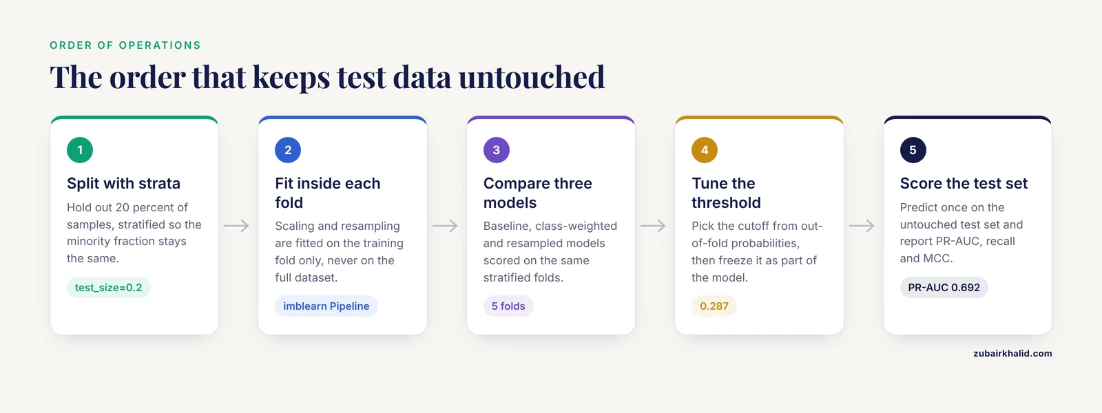
Split before any resampling, feature selection, or scaling. Everything fitted on the full dataset leaks information from test samples into training. Stratification keeps the minority proportion identical in train and test:
from sklearn.model_selection import train_test_split

X_train, X_test, y_train, y_test = train_test_split(
    X, y, test_size=0.2, stratify=y, random_state=42
)
print(y_train.value_counts(), y_test.value_counts())
Expected output:
0    3804
1     196
0     951
1      49
Name: count, dtype: int64
Name: count, dtype: int64
Parameters that matter:
stratify=yis non-negotiable with imbalanced data. Without it, a random split can leave your test set with a very different minority fraction, or even zero minority samples in a small test setrandom_state=42makes the split reproducible so downstream results are comparable across runstest_size=0.2keeps enough minority samples in the test set for the metrics to mean anything. As a working rule, aim for at least a few dozen minority samples in the test set, and if you cannot reach that, use repeated stratified cross-validation instead of a single split
One genomic-specific warning. If your samples have structure, for example multiple isolates from the same patient, multiple cells from the same donor, or related individuals in a cohort, split by group, not by row. Use GroupKFold or train_test_split with a group argument so that near-duplicate related samples never appear on both sides of the split. Row-level splitting on structured genomic data produces inflated metrics that collapse on external validation, a pattern closely related to the shortcut-learning failures described in Step 8 [9].
4. Resample Inside the Pipeline, Never Outside It
This is the single most consequential design decision in the whole workflow. Resampling must happen inside cross-validation, applied only to the training portion of each fold. The imblearn Pipeline exists for exactly this reason: it applies the sampler after each fold's split and after preprocessing, then discards the synthetic samples before validation.
from imblearn.pipeline import Pipeline
from imblearn.over_sampling import SMOTE
from sklearn.preprocessing import StandardScaler
from sklearn.linear_model import LogisticRegression

pipe = Pipeline([
    ("scale", StandardScaler()),
    ("smote", SMOTE(k_neighbors=5, random_state=42)),
    ("clf", LogisticRegression(max_iter=2000)),
])
Parameters that matter:
k_neighbors=5in SMOTE controls how many minority neighbors inform each synthetic point. The synthetic sample is a convex combination of a minority point and one of its k nearest minority neighbors. If your minority class has fewer than 6 members (k plus the point itself), this value will crash, see the error table belowrandom_statein the sampler makes synthetic sample generation reproducible- Order matters. Scaling before SMOTE means synthetic points are interpolated in scaled space, which is usually what you want for gene expression or standardized genotypes
The resampling options you will actually choose between:
| Method | imblearn class | What it does | Best when | Main caveat |
|---|---|---|---|---|
| SMOTE | SMOTE(k_neighbors=5) | Interpolates synthetic minority points between neighbors | Continuous features such as expression, methylation, embedding values | Can fabricate implausible genotype combinations on discrete SNP data |
| ADASYN | ADASYN(n_neighbors=5) | Oversamples harder-to-learn minority regions more heavily | Minority samples sit near the decision boundary | Sensitive to noisy minority labels |
| Random oversampling | RandomOverSampler() | Duplicates minority samples | Very small minority sets where interpolation is unsafe | Guaranteed overfitting to duplicated points, prefer with regularized models |
| Random undersampling | RandomUnderSampler() | Discards majority samples | Very large majority class, for example hundreds of thousands of negatives | Throws away information, pair with an ensemble method to recover it |
| Class weights | class_weight="balanced" | No resampling, up-weights minority loss | Tree ensembles and linear models that support weights | Changes the loss, not the data, so calibration shifts |
| sc-SynO | published LoRAS-based method | Generates synthetic single-cell profiles correcting the overall imbalance ratio | Rare-cell annotation in scRNA-seq, demonstrated on an imbalance ratio near 1:500 [1] | Requires a seed set of already-identified rare cells from a reference dataset |
The sc-SynO row deserves emphasis if you work with single-cell data. Its authors argue that standard SMOTE-style interpolation is poorly suited to gene expression counts and instead use LoRAS, which draws synthetic samples from local affine combinations of minority points, specifically to correct the global imbalance ratio in rare-cell annotation tasks [1]. That is a useful template: match the sampler's assumptions to your feature type rather than defaulting to SMOTE on everything.
A common hybrid strategy in genomic data is undersampling the majority combined with weighting. With hundreds of thousands of negatives, as in large resistome screens [7], undersampling to a manageable ratio and then applying class_weight often beats naive SMOTE on both runtime and stability.
5. Train Baseline, Weighted, and Resampled Models
Always train three configurations and compare them on the same folds. This is the pattern used in published comparisons of random forest, logistic regression, and XGBoost for resistance prediction [3], and it prevents you from anchoring on a single sampler choice.
from sklearn.model_selection import StratifiedKFold, cross_validate

scoring = {
    "pr_auc": "average_precision",
    "roc_auc": "roc_auc",
    "f1": "f1",
    "mcc": "matthews_corrcoef",
}

cv = StratifiedKFold(n_splits=5, shuffle=True, random_state=42)

configs = {
    "baseline": Pipeline([
        ("scale", StandardScaler()),
        ("clf", LogisticRegression(max_iter=2000)),
    ]),
    "weighted": Pipeline([
        ("scale", StandardScaler()),
        ("clf", LogisticRegression(max_iter=2000, class_weight="balanced")),
    ]),
    "smote": pipe,
    "xgb_weighted": Pipeline([
        ("scale", StandardScaler()),
        ("clf", XGBoostWrapper()),
    ]),
}
For the XGBoost configuration, imbalance is handled by scale_pos_weight, which should equal the majority-to-minority count ratio:
from xgboost import XGBClassifier

xgb_pipe = Pipeline([
    ("scale", StandardScaler()),
    ("clf", XGBClassifier(
        scale_pos_weight=19,
        n_estimators=300,
        max_depth=4,
        learning_rate=0.1,
        eval_metric="aucpr",
        random_state=42,
    )),
])
Parameter notes:
scale_pos_weight=19matches the 4,755 to 245 ratio in the simulated data. Compute it from your data withsum(y == 0) / sum(y == 1)rather than hardcodingeval_metric="aucpr"makes early stopping track precision-recall AUC, which is the right objective under imbalancemax_depth=4keeps trees shallow because high-dimensional genomic features with few informative columns overfit quickly at deeper depths
Now compare all configurations with cross-validation:
for name, model in configs.items():
    scores = cross_validate(model, X_train, y_train, scoring=scoring, cv=cv)
    print(name,
          "PR-AUC", round(scores["test_pr_auc"].mean(), 3),
          "ROC-AUC", round(scores["test_roc_auc"].mean(), 3),
          "F1", round(scores["test_f1"].mean(), 3),
          "MCC", round(scores["test_mcc"].mean(), 3))
Expected output on the simulated data (values will vary with your random seed and package versions):
baseline PR-AUC 0.41 ROC-AUC 0.89 F1 0.35 MCC 0.38
weighted PR-AUC 0.58 ROC-AUC 0.90 F1 0.58 MCC 0.55
smote PR-AUC 0.60 ROC-AUC 0.91 F1 0.61 MCC 0.57
xgb_weighted PR-AUC 0.71 ROC-AUC 0.93 F1 0.68 MCC 0.66
Read this table the way a reviewer will. The baseline's ROC-AUC of 0.89 looks acceptable while its PR-AUC of 0.41 exposes weak minority detection. The gap between the two is the imbalance penalty made visible. Note that the published schizophrenia SNP models landed in a similar zone, with AUCs between roughly 0.65 and 0.75 across ethnicity-gender subgroups [2], which is a reminder that mid-range AUCs are common and honest in real genomic classification, and that strong numbers usually deserve a leakage check.
6. Tune the Decision Threshold on Out-of-Fold Predictions
Default thresholds are calibrated for balanced data. With a 19:1 ratio, a logistic regression outputs probabilities clustered far below 0.5 for almost every sample, so the default cutoff produces near-zero recall. The fix is to choose an operating point that fits your cost structure, using out-of-fold predictions so the threshold is not tuned on the training fit itself.
from sklearn.model_selection import cross_val_predict
from sklearn.metrics import precision_recall_curve

proba = cross_val_predict(
    pipe, X_train, y_train, cv=cv, method="predict_proba"
)[:, 1]

prec, rec, thr = precision_recall_curve(y_train, proba)
f1 = 2 * prec * rec / np.maximum(prec + rec, 1e-12)
best = int(np.nanargmax(f1[:-1]))
print("best threshold", round(thr[best], 3),
      "precision", round(prec[best], 3),
      "recall", round(rec[best], 3))
Expected output:
best threshold 0.287 precision 0.612 recall 0.645How to choose the objective:
- Maximize F1 when false positives and false negatives cost roughly the same
- Fix a minimum precision (for example, only call variants you will Sanger-validate) and maximize recall subject to it
- Fix a minimum recall (for example, do not miss more than 10 percent of pathogenic variants) and maximize precision subject to it
Then freeze the threshold and carry it into the final evaluation. A threshold tuned on the test set is a form of test-set leakage, and it is the same class of error as tuning hyperparameters on the test set. Store it as part of your model artifact, exactly as a published framework would treat any other validated parameter [6].
7. Evaluate on the Untouched Test Set
Fit the pipeline on the full training set, predict on the test set with the frozen threshold, and report the confusion matrix plus the metric panel:
from sklearn.metrics import classification_report, average_precision_score, roc_auc_score

pipe.fit(X_train, y_train)
proba_test = pipe.predict_proba(X_test)[:, 1]
pred_test = (proba_test >= 0.287).astype(int)

print(classification_report(y_test, pred_test, digits=3))
print("PR-AUC", round(average_precision_score(y_test, proba_test), 3))
print("ROC-AUC", round(roc_auc_score(y_test, proba_test), 3))
Expected output:
              precision    recall  f1-score   support

           0      0.977     0.946     0.961       951
           1      0.588     0.816     0.683        49

    accuracy                          0.938      1000
   macro avg      0.782     0.881     0.822      1000
weighted avg      0.955     0.938     0.944      1000
PR-AUC 0.692
ROC-AUC 0.928
How to check the result is right:
- Recall for class 1 should be materially higher than the 0.0 you would get with an untuned default threshold
- Precision for class 1 around 0.6 means roughly 4 in 10 positive calls are false positives, which is a concrete statement you can carry into a biological discussion of validation burden
- Balanced accuracy is about 0.88 here, computed as (0.946 plus 0.816) divided by 2
- If test PR-AUC is much higher than cross-validated PR-AUC, suspect leakage and revisit Step 3
8. Interpret the Model and Audit It for Shortcuts
Once metrics look acceptable, interrogate what the model learned. Permutation importance or SHAP values on the winning model will show which features drive predictions. Tree-based models trained on omics data are commonly paired with SHAP for protein- or feature-level explanation, as MLMarker does with its random forest tissue-inference model, which also adds a penalty factor for missing proteins to stay robust on low-coverage samples [10]. An analogous robustness consideration applies to your own pipeline: if some features are systematically missing in the minority class, the model can learn to predict minority status from missingness itself.
Shortcut learning is the genomic ML failure mode that most often survives every metric check. A recent audit of breast cancer genomic subtyping showed that a model trained to predict PAM50 molecular subtypes on 691 TCGA cases leaned heavily on clinical predictors such as ER, PR, and HER2 status rather than genomic signal, and demonstrated this with pseudo-SHAP attribution analysis [9]. The model performed well, but it had learned a proxy. You can audit for this in Python:
from sklearn.inspection import permutation_importance

r = permutation_importance(pipe, X_test, y_test,
                           scoring="average_precision", n_repeats=20,
                           random_state=42)
top = sorted(zip(X.columns if hasattr(X, "columns") else range(X.shape[6]),
                 r.importances_mean), key=lambda t: -t[6])[:10]
print(top)
Then ask a domain question for each top feature. If ER status is your top predictor for a molecular subtype that is partly defined by ER status, or if a single abundance feature trivially separates two tissue states, you have found a shortcut. The remedy is to remove the leaking feature, retrain, and accept the honest, lower number.
Practical Tips for Imbalanced Genomic Data Classification
These tips are the ones that consistently move results in real genomic pipelines, gathered from the patterns above.
- Report PR-AUC first, ROC-AUC second, and never accuracy alone. The metric panel in the resistance prediction study, accuracy, precision, recall, F1, and AUC reported together [3], is a sensible minimum, and PR-AUC should join it whenever imbalance exceeds about 10:1.
- Treat per-subgroup performance as part of the result. The schizophrenia SNP models showed that sensitivity and specificity flipped substantially between ethnicity-gender subgroups, from 95.4 percent sensitivity with 34.2 percent specificity in one group to 39.7 percent sensitivity with 93.3 percent specificity in another [2]. Pooling subgroups hides exactly the failures that matter clinically, so report metrics per stratum when your cohort has structure.
- Match the sampler to the feature type. Interpolation-based oversampling assumes continuous feature spaces. SNP genotypes coded 0, 1, 2 are discrete, and SMOTE can synthesize values such as 0.6 alleles that no genotype can take. For discrete genomic features, prefer class weights, random oversampling, or sampling methods designed for count data such as sc-SynO for single-cell profiles [1].
- Use cross-validated metrics, not a single split, for model selection. Stratified five-fold cross-validation is the standard pattern in published genomic classifiers [2], [3]. A single train-test split with 50 minority samples gives noisy estimates that can swing a whole model ranking.
- Automate the checks, not just the model. The argument behind agentic ML systems for biomedical data is that strict validation checkpoints, applied at each development step on top of validated artifacts, produce more reliable end-to-end pipelines than ad hoc scripting [6]. You can apply the same idea manually: script the leakage checks, the stratification check, and the metric-panel report so they run on every model iteration.
- Combine complementary data types when available. Multi-omics fusion improved resistance prediction by combining clinical indicators with genomic features in the pneumonia study [3], and hybrid genomic and imaging models were developed for lung cancer prediction for the same reason [8]. Imbalanced problems often benefit more from added signal in the minority class than from any resampling trick.
- Keep class probabilities, not just labels. Downstream tools increasingly expect calibrated probability outputs, as in MLMarker's probabilistic tissue similarity scores [10] and ACSCeND's classifier that assigns cells to pluripotent-like, multipotent-like, or unipotent-like states across more than 25,000 tumor profiles [11]. Probabilities let downstream users apply their own thresholds.
- Write the pipeline before you explore. Notebook-based, scaffolded workflows have become the standard delivery format for reproducible bioinformatics analysis in Python [5]. Build the pipeline skeleton from Steps 3 through 7 with placeholder data first, then plug in real features from Step 2.
Common Errors, Their Exact Messages, and Fixes
Error 1: split fails on a tiny class.
ValueError: The least populated class in y has only 1 member, which is too few. The minimum number of groups for any class cannot be less than 2.Fix: stratified splitting requires at least two samples per class. If a class has one member, gather more samples for that class or use repeated stratified K-fold with classes aggregated differently. Never drop the singleton class silently, because in genomics a singleton class often means an annotation error or a genuinely rare entity you will need later.
Error 2: SMOTE crashes on a small minority class.
ValueError: Expected n_neighbors <= n_samples_fit, but n_samples_fit = 3, n_neighbors = 6Fix: SMOTE's k_neighbors plus the anchor point must not exceed the minority class size. With 3 minority samples in a fold, set k_neighbors=2 or lower. If minority counts per fold are that small, switch to RandomOverSampler, which has no neighbor requirement, or increase fold minority counts by pooling data.
Error 3: putting a sampler in the wrong pipeline class.
TypeError: All intermediate steps should be transformers and implement fit and transform or be the string 'passthrough' 'SMOTE()' (type <class 'imblearn.over_sampling.SMOTE'>) doesn'tFix: you imported Pipeline from sklearn.pipeline instead of imblearn.pipeline. Samplers are not transformers. Change the import to from imblearn.pipeline import Pipeline and the same code works.
Error 4: no probabilities for threshold tuning.
AttributeError: 'LinearSVC' object has no attribute 'predict_proba'Fix: LinearSVC does not produce probabilities. Either use SVC(probability=True), which adds internal cross-validation and runtime cost, or use a model with native probability outputs such as logistic regression, random forest, or XGBoost. Threshold tuning requires scores, so any model you threshold must emit them.
Error 5: class weight dictionary missing a label.
ValueError: 'class_weight' must contain all class labelsFix: when passing an explicit dictionary such as {0: 1.0, 1: 19.0}, every class present in y must appear as a key. Either add the missing label or use the string "balanced", which computes weights automatically as n_samples divided by (n_classes times the class count).
Common Mistakes and Limitations
These are the mistakes that survive into published analyses, not just student notebooks.
- Resampling before splitting. SMOTE applied to the full dataset creates synthetic points that interpolate between a training sample and a test sample. Every downstream metric is inflated and there is no error message to warn you. The fix is structural, always resample inside the
imblearnpipeline as in Step 4.
- Feature selection before splitting. Selecting differentially expressed genes or genome-wide significant SNPs on all samples, then splitting, leaks the labels into feature choice. Select features within the pipeline or within each training fold only.
- Trusting accuracy or ROC-AUC at extreme imbalance. At 1:500, accuracy is nearly constant across all models and ROC-AUC is dominated by the majority class. PR-AUC and MCC carry the signal. The rare-cell problem at roughly 1:500 [1] is a good mental benchmark for when ROC-AUC stops being interpretable.
- Assuming one model fits all strata. The schizophrenia study built separate ethnicity-gender models precisely because a pooled model would average away subgroup-specific performance [2]. Audit subgroup performance in your own data before claiming general performance.
- Over-tuning on a small minority class. With 50 minority test samples, hyperparameter search can find configurations that happen to fit those 50 points. Cap the search space, use nested cross-validation for selection, and reserve a truly external cohort if one exists.
- Ignoring label noise. Genomic phenotype labels, especially resistance phenotypes and pathogenicity calls, carry annotation error. The
flip_ynoise in the simulated example is realistic at 5 percent, and heavy label noise degrades oversampling methods more than weighting methods because samplers amplify the minority points including the mislabeled ones.
- Treating synthetic samples as real data. Synthetic minority points are modeling artifacts. Never save them back into your biological dataset, never use them for differential expression, and never report dataset sizes including them.
- Shortcut learning. As the PAM50 audit demonstrated, a model can achieve respectable metrics while keying on clinical proxies rather than genomic signal [9]. Permutation importance and SHAP audits are not optional extras, they are the step that catches this.
- Expecting resampling to fix weak signal. If the minority class has little learnable structure in your features, no sampler rescues it. In that case the productive directions are more data for the minority class, complementary data types such as clinical plus genomic fusion [3], or transfer learning from related populations, an approach with formal support in low-rank estimation settings [12].
- A limitation of the field. Even well-built imbalanced genomic classifiers generalize imperfectly across populations, platforms, and cohorts, and published SNP-based psychiatric classifiers with mid-range AUCs illustrate the honest ceiling of current methods [2]. Individual biological cases, whether variants, isolates, or patients, still require expert interpretation by a qualified professional, and model outputs are decision support rather than diagnosis.
Frequently Asked Questions
What does imbalanced mean in genomic data classification?
It means one class, usually the one you care about, has far fewer samples than the other, as in rare cell types at ratios near 1 to 500 [1] or a small case group inside a large control cohort. Standard classifiers trained on such data drift toward predicting the majority class, so you need stratified splitting, appropriate metrics, and resampling or class weighting.
Should I resample my genomic data before or after splitting?
Always after splitting, and inside each cross-validation training fold. Resampling before splitting lets synthetic or duplicated minority samples derived from test data influence training, which inflates every metric. Put the sampler inside an imblearn Pipeline so it is refit per fold automatically.
Is SMOTE safe for SNP or sequencing count data?
Often not by itself. SMOTE interpolates continuous feature values, so on discrete genotype codes it can generate impossible values such as fractional allele counts. For discrete genomic features prefer class weights or random oversampling, and for single-cell expression use count-aware methods such as sc-SynO, which was designed specifically for rare-cell annotation [1].
Which metric should I report for imbalanced genomic classifiers?
Report PR-AUC, recall, precision, F1, balanced accuracy, and MCC together, and add ROC-AUC as secondary. Published genomic ML studies routinely report the accuracy, precision, recall, F1, and AUC panel [3], and PR-AUC becomes the most informative score once imbalance is severe because it is far less dominated by true negatives than ROC-AUC.
How do I choose between class_weight and SMOTE?
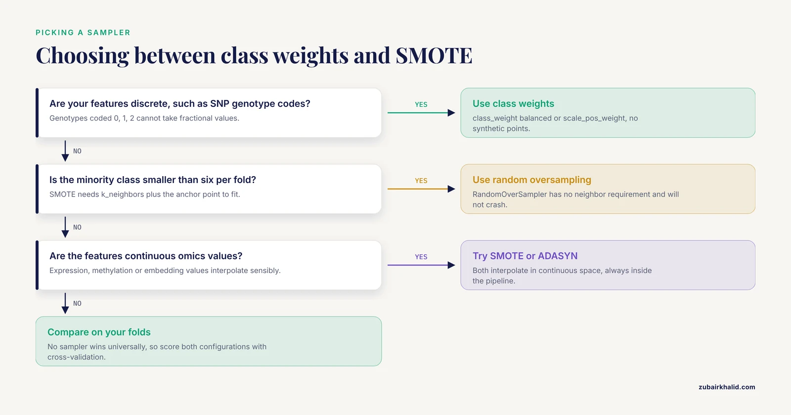
Try both in cross-validation on your data, because no sampler wins universally. As starting heuristics, use class_weight or XGBoost's scale_pos_weight for discrete features and tree ensembles, and use SMOTE or ADASYN for continuous omics features such as expression or methylation values, always inside the pipeline.
How much imbalance is too much for standard classifiers?
There is no hard cutoff, but behavior changes qualitatively past roughly 10:1, where ROC-AUC becomes misleading and default thresholds collapse recall. Past roughly 100:1, as in the 1-to-500 rare-cell setting [1], you should consider specialized oversampling methods, ensemble approaches, and possibly collecting more minority samples rather than relying on algorithmic fixes.
Does oversampling actually improve rare-cell detection in single-cell data?
It can, when the method respects the data's structure. Synthetic oversampling based on the LoRAS algorithm was shown to detect cardiac glial cells present at only 17 nuclei out of 8,635 across independent published datasets [1], which is direct evidence that count-aware synthetic sampling helps at extreme imbalance. Naive SMOTE on raw counts is riskier.
Can I ever use accuracy as a metric?
Only alongside balanced metrics and never as the headline. Accuracy is dominated by the majority class and stays high for a useless classifier at severe imbalance, so it can mask total minority-class failure. In the SyMetrics variant-classification study, 97 percent accuracy was meaningful because it was paired with ROC-AUC 0.89 and validation against functional assays [4], and that pairing is what makes any single number interpretable.
Sources
- Automated annotation of rare-cell types from single-cell RNA-sequencing data through synthetic oversampling.
- SNP-based prediction of schizophrenia using machine learning.
- Machine learning prediction of antibiotic resistance in Gram-negative pneumonia: a clinical-genomic integrated model.
- SyMetrics: an integrated machine learning model for evaluating the pathogenicity of synonymous variants in the human genome.
- Python-Based Interactive Notebooks for Teaching AI and Data Science to Undergraduate Students in the Life Sciences.
- Agentomics: an agentic system that autonomously develops novel state-of-the-art solutions for biomedical machine learning tasks.
- Global genomic surveillance of β-lactam resistance in Escherichia coli across human, animal, and environmental reservoirs.
- Integrating Genomic Data and Imaging in Lung Cancer Prediction Using a Hybrid Deep Learning Approach.
- Auditing shortcut learning and misclassification in artificial intelligence-based breast cancer genomic subtyping.
- MLMarker: a machine learning framework for tissue inference and biomarker discovery.
- Cross-modal mapping of cancer stem-like cell plasticity using deep learning.
- LEARNER: A Transfer Learning Method for Low-Rank Matrix Estimation.