How to Evaluate Genomic Classifiers in Python
By Dr. Zubair Khalid, DVM, MS, PhD ·

Evaluating a genomic classifier means measuring how reliably it assigns labels to genomic data it has never seen, while building the classifier means fitting the model to data it has already seen. The two are separate jobs, and most published models fail at the second one. The rule of thumb is simple: if your headline number changes noticeably when you change the random seed or the data split, you are reporting noise, and you should spend your effort on validation design before you touch model choice at all.
This guide walks through the full evaluation workflow in Python, from loading genomic matrices to reporting defensible numbers. It covers the library options and their pros and cons, the metrics that matter for genomic data, validation designs that survive peer review, worked code, and the mistakes that most often invalidate results.
What Evaluating a Genomic Classifier Actually Involves
A genomic classifier is any model that assigns a discrete label to a biological sample or sequence. Common examples include tumor subtype assignment from gene expression, resistant versus susceptible calls from bacterial genomes, pathogenic versus benign labels for genetic variants, and cell state annotations in single-cell data. The input is usually a matrix of features (gene expression values, SNP genotypes, k-mer counts, variant annotations) and the output is a predicted class or a probability.
Evaluation has three distinct parts, and conflating them is the root of most bad results:
- Generalization performance. How accurate is the model on samples drawn from the same population but not used in training? This is what cross-validation and held-out test sets estimate.
- Fitness for purpose. A classifier with 97% accuracy can still be useless if it misses exactly the cases you care about. The SyMetrics framework for synonymous variant pathogenicity, for example, reports 97% accuracy and a ROC-AUC of 0.89, but its real value is judged by whether predicted damaging variants are confirmed in functional assays and clinical cohorts, which the authors checked experimentally [1].
- Stability and reproducibility. Does the model give the same answer twice? Do the same features drive predictions across resampling? The protein interaction hot spot work by Chen, Kuhn, and Raschka treats repeated repartitioning of training and test sets as the single most telling experiment, because it shows whether a classifier performs consistently rather than luckily on one split [2].
A proper evaluation answers all three. A poor one reports a single accuracy figure from one convenient split.
Why Python Is the Default for This Work
Python has become the standard language for bioinformatics machine learning for practical reasons. The scikit-learn library provides a consistent interface to dozens of classifiers, resampling schemes, and metrics, which means a logistic regression and a random forest are evaluated with identical code and therefore identical rigor. Recent literature reflects this. The clinical-genomic model for antibiotic resistance in Gram-negative pneumonia built its random forest, logistic regression, and XGBoost models in Python 3.9 [3]. MLMarker ships as a Python package with a Streamlit app [4]. Profylo, pyVIPER, and aPhyloGeo are all released as open-source Python tools [5][6][7].
Two properties of the Python ecosystem matter most for evaluation specifically:
- Pipelines enforce correctness. Scikit-learn pipeline objects bundle preprocessing and the model into one object, so cross-validation refits the scaler on each training fold. This prevents a subtle and extremely common form of data leakage discussed later.
- Interoperability. Tools like pyVIPER integrate directly with scverse, scanpy, and standard machine learning libraries, so a classifier built on single-cell data plugs into the same evaluation machinery as one built on bulk expression [7].
R remains a strong ecosystem for statistical genomics, and the melanoma multi-omics fusion study developed its methods in both R and Python [8]. For classifier evaluation specifically, Python's advantage is that the same code path handles preprocessing, model fitting, resampling, and metric computation, which removes most opportunities for inconsistency.
Your Evaluation Toolkit: Options Compared
The main options for evaluating genomic classifiers in Python, and how they trade off against each other, are summarized below.
| Option | Best for | Strengths | Drawbacks |
|---|---|---|---|
| scikit-learn | Tabular omics data (expression, variant features, k-mer counts) | One consistent API, pipelines that prevent leakage, built-in cross-validation and metrics | Memory limits on very wide matrices, no native GPU or deep learning support |
| XGBoost and LightGBM | Mixed feature types, nonlinear interactions, moderate sample sizes | Strong tabular performance, native handling of missing values, feature importance | Heavy tuning burden, easy to overfit small noisy omics datasets |
| PyTorch | Sequence data, deep architectures, very large datasets | Flexible architectures, GPU acceleration, foundation model support | Needs much more data, harder to validate rigorously, more code to get wrong |
| Biopython | Data preparation from biological file formats | Standard parsers for FASTA, GenBank, alignment files, BLAST output | Not a machine learning library, no modeling or metrics |
| scverse and scanpy | Single-cell classifiers and state annotation | De facto standard for single-cell workflows, integrates with sklearn and PyTorch | Large memory footprint, results sensitive to preprocessing choices |
| SHAP and permutation importance | Explaining predictions after evaluation | Model-agnostic attribution, now used in production genomics tools | Slow on large models, misleading when features are correlated |
| Automated pipelines and agentic systems | End-to-end experimentation at scale | Enforces validation checkpoints, improves reproducibility | Less fine-grained control, output still requires expert review |
Each option deserves a closer look, because the pros and cons decide real choices in genomic projects.
scikit-learn as the Evaluation Backbone
For most genomic classification problems, where the input is a samples-by-features matrix, scikit-learn is the right backbone regardless of which final model you choose. Its value for evaluation is not that its models are best, but that its evaluation machinery is uniform. cross_validate runs the same resampling, the same refitting, and the same scoring across any estimator, so comparisons between models are apples to apples.
Chen, Kuhn, and Raschka's protocol for protein interaction hot spot prediction leans on exactly this property, using scikit-learn to compare several classifiers on a curated dataset of 1046 non-redundant alanine scanning mutation sites and to assess whether enough data has been used for training [2]. That paper is a good template for rigorous small-data evaluation in Python.
The main limitation is scale. scikit-learn loads everything into memory, so a matrix of 10,000 tumors by 60,000 transcripts is manageable, while single-nucleotide-resolution data across a whole genome generally is not.
Gradient Boosting with XGBoost
XGBoost earned its place in the antibiotic resistance study alongside logistic regression and random forest as one of the three benchmarked models [3]. Its practical advantages for genomic data are native handling of missing values (common in clinical-genomic merges) and its tolerance for mixed feature types without extensive preprocessing. The drawback is tuning: gradient boosted trees have more hyperparameters than a regularized logistic regression, and every hyperparameter search must happen inside the cross-validation loop or it leaks information. In the pneumonia study the three models were compared on accuracy, precision, recall, F1 score, and AUC, with calibration and decision curves added to judge clinical usefulness [3], which is the metric panel you should imitate for clinical applications.
PyTorch for Sequence-Level Models
When the classifier consumes raw sequence rather than a fixed feature matrix, deep learning enters. DeepHyb, a convolutional neural network for inferring hybridization events, combines four complementary feature representations drawn from multiple sequence alignments, including 15 summary site patterns, 256 one-base site patterns, 75 summary k-mer patterns, and 256 sequence-level k-mer patterns [9]. simcat trains a neural network on coalescent simulations to discriminate introgression scenarios from SNP frequency patterns across all quartets simultaneously [10]. AESTETIK learns joint representations of spatial, transcriptomic, and morphology data in spatial transcriptomics [11].
The pros are the ability to learn feature interactions you would never hand-engineer, and mature GPU acceleration. The cons are that evaluation gets harder, not easier. Deep models need larger validation sets to produce stable estimates, they are prone to overfitting genomic datasets that have more features than samples, and their interpretability requires extra tooling, as DeepCC9 had to build explicit feature extraction into its architecture specifically to recover the sequence motifs governing CRISPR-Cas9 efficiency [12].
Biopython for Data Preparation
Biopython is not an evaluation library, but genomic classifier projects usually start with sequences in FASTA or GenBank files, and Biopython is the standard Python interface to those formats. A minimal Biopython tutorial-style example that turns sequences into k-mer features suitable for scikit-learn looks like this:
from Bio import SeqIO
from collections import Counter

def kmer_counts(fasta_path, k=3):
    counts = Counter()
    for record in SeqIO.parse(fasta_path, "fasta"):
        seq = str(record.seq).upper()
        for i in range(len(seq) - k + 1):
            counts[seq[i:i + k]] += 1
    return counts
The clean division of labor is that Biopython converts biological files into Python data structures, pandas assembles them into a feature matrix, and scikit-learn does the modeling and evaluation. Problems arise when people blur those boundaries, for example by computing features with inconsistent k-mer definitions across runs, which silently invalidates comparisons.
The Single-Cell Ecosystem
Single-cell classifiers have their own tooling. ACSCeND, a machine learning framework that classifies cancer stem-like cell states from single-cell RNA-seq data and deconvolves those states from bulk RNA-seq, was applied to more than 25,000 tumor profiles from TCGA, PRECOG, relapse, and immunotherapy studies [13]. pyVIPER, which infers protein activity from single-cell transcriptomic data, uses PyTorch-based GPU acceleration to cut large-dataset analysis times from hours to minutes and integrates with scanpy and the wider scverse ecosystem [7].
For evaluation, the single-cell wrinkle is that samples are cells, and cells from the same patient are not independent. If you split at the cell level, your cross-validation folds share patients, and your accuracy estimate is optimistic. Split at the patient level.
Interpretability Tools
Modern genomic classifiers are increasingly expected to explain themselves. MLMarker pairs its random forest tissue classifier with SHAP-based protein-level explanations so users can see which proteins drive a tissue assignment [4]. DeepCC9 combines explicit sequence feature extraction with a residual block-based deep architecture specifically to identify the 74 sequence motifs enriched or depleted at particular positions within sgRNAs [12].
Interpretability tools are part of evaluation because a classifier whose explanations contradict known biology should not ship, no matter what its AUC says. The caveat is that SHAP values and importances are misleading when features are correlated, which is the norm in genomics, where thousands of genes move together. Treat attributions as hypotheses for follow-up, not proof of mechanism.
Automated and Agentic Pipelines
The newest option is automated experimentation. Agentomics is an LLM-powered agentic system that takes a biomedical dataset, implements multiple machine learning modeling strategies, and produces a ready-to-use model, with strict validation checkpoints at each standard development step so that progress builds on validated artifacts. It was evaluated across 20 datasets spanning protein engineering, drug discovery, and regulatory genomics [14]. For a lab without dedicated machine learning staff, this class of tool can produce a defensible baseline evaluation quickly. The tradeoff is control. You should inspect the validation design an automated system chose, because automation does not remove the obligation to check for leakage or inappropriate splits.
Metrics That Actually Matter for Genomic Data
Threshold Metrics: Accuracy, Precision, Recall, F1
Accuracy, precision, recall (also called sensitivity), specificity, and the F1 score are all computed at a fixed decision threshold. They answer the question "at this cutoff, how often is the classifier right?" The pneumonia resistance study reported all of these for its three models [3], and SyMetrics reported 97% accuracy for distinguishing deleterious from benign synonymous variants [1].
These numbers are easy to communicate and easy to misuse. In genomics, the two failure modes are:
- Imbalanced classes make accuracy meaningless. A classifier that predicts "benign" for every variant in a dataset that is 99% benign scores 99% accuracy while being worthless.
- Sensitivity and specificity trade off against each other, and the tradeoff point depends on the threshold. The schizophrenia SNP prediction study illustrates this sharply. Its ethnicity and gender specific models achieved, for example, 75.1% accuracy in the European-American female group, but with an AUC of 69.2%, sensitivity of 95.4%, and specificity of only 34.2%. A model tuned to catch nearly all cases misses most controls. Reporting accuracy alone would have hidden this entirely.
Always report the full confusion matrix or at minimum sensitivity and specificity together with a stated threshold.
Ranking Metrics: ROC-AUC
ROC-AUC (the area under the receiver operating characteristic curve, which plots true positive rate against false positive rate across all thresholds) measures how well the model ranks cases above controls, independent of any threshold. It is the most commonly reported single number in genomic classification, appearing in SyMetrics (0.89) [1], the schizophrenia models [15], and the pneumonia study [3].
Its limitation is that ROC-AUC treats false positives and false negatives as equally costly, which is rarely true clinically. A screening classifier that misses a pathogenic variant is worse than one that raises a false alarm, and ROC-AUC cannot express that asymmetry. Precision-recall curves are more informative when the positive class is rare.
Calibration and Decision-Curve Analysis

If the classifier outputs probabilities that clinicians or researchers will act on, ranking is not enough. A model that says a tumor has a 0.7 probability of subtype A should be right about 70% of the time. Calibration curves assess this, and decision curve analysis asks whether acting on the model's probabilities produces better decisions than default strategies across a range of threshold preferences. The antibiotic resistance study evaluated exactly this way, verifying clinical applicability through calibration curves and decision curves in addition to the standard metrics [3]. For any classifier intended to inform a decision rather than just rank samples, include both.
Multiclass Settings
Tumor subtyping and cell state annotation are usually multiclass. Report macro-averaged metrics (which weight each class equally) rather than micro-averaged ones (which weight each sample equally), because the rare class is usually the interesting one. ROC-AUC extends to multiclass via one-vs-one or one-vs-rest averaging, and scikit-learn supports both.
Validation Design: Where Most Evaluations Fail
Model choice is rarely what separates a trustworthy genomic classifier from an untrustworthy one. Validation design is.
Stratified k-Fold Cross-Validation
Stratified k-fold cross-validation partitions the data into k folds while preserving class proportions in each fold, trains on k minus 1 folds, and tests on the held-out fold, rotating until every sample has been tested exactly once. The schizophrenia SNP study based model selection on stratified five-fold cross-validation [15]. Five folds is a common default. Ten folds gives a slightly less variable estimate at higher compute cost.
For small genomic datasets, repeat the process. The hot spot protocol used 500-fold repartitioning of training and test sets followed by prediction on each repartition, giving a direct read on whether performance is consistent across different splits rather than an artifact of one lucky partition [2]. Twenty to fifty repetitions of five-fold cross-validation is a reasonable practical target, and the standard deviation across repetitions belongs in your report.
External Validation on Independent Data
Cross-validation estimates performance within a dataset. It cannot tell you whether the model transfers to a different cohort, sequencing platform, or population. The federated learning study on variant pathogenicity annotation found that models trained across multiple institutions achieved robust generalization to independent sets, and in some cases better generalization, than centralized models trained on pooled data [16]. The mechanism matters here: exposing the model to several institutions' data during training made it less dependent on any one cohort's quirks.
The practical rule is that a genomic classifier intended for real use needs at least one truly external test set, processed independently of training data. If you cannot get one, say so plainly in your results.
Preventing Leakage
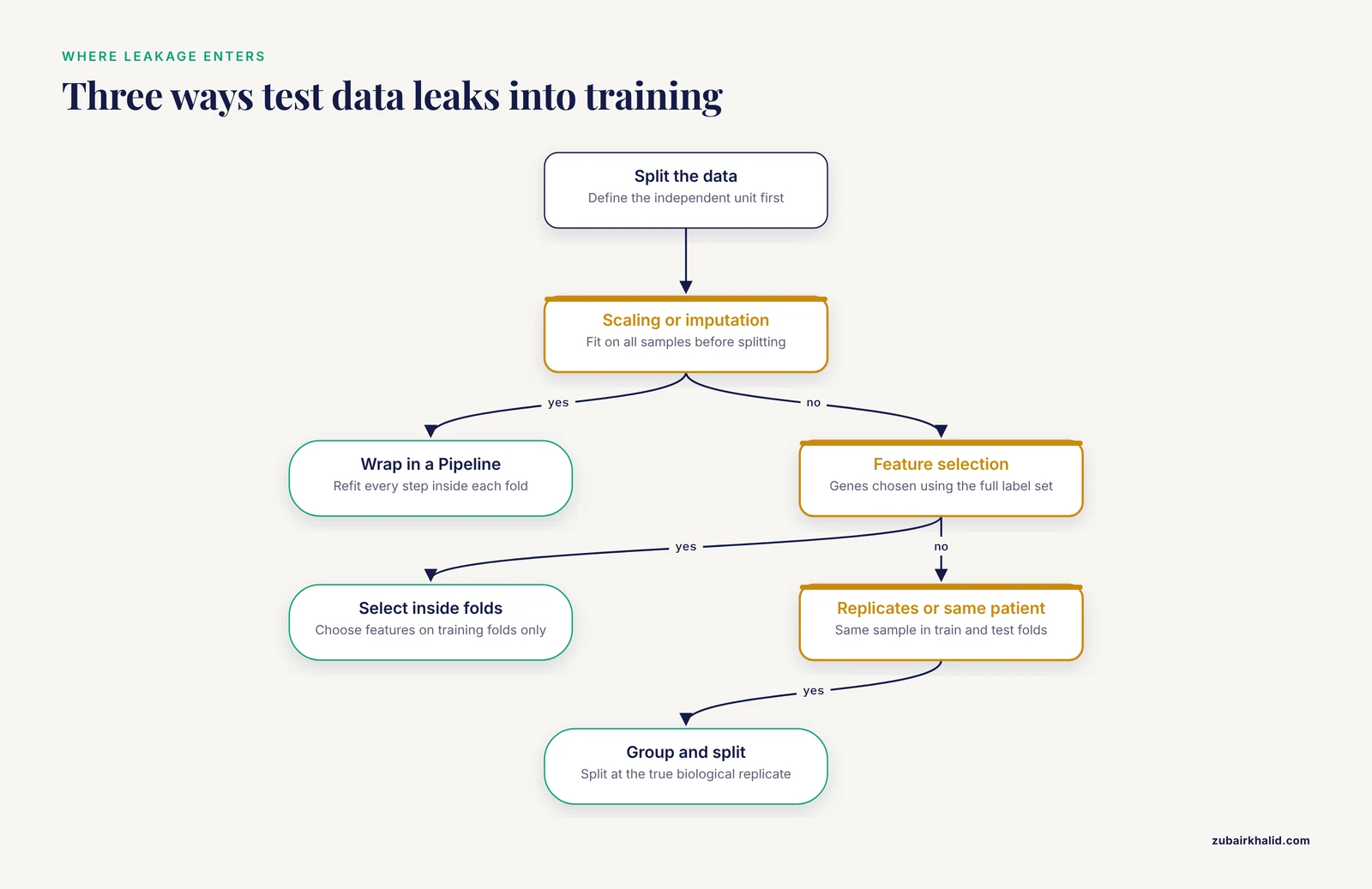
Data leakage, where information from the test set influences training, is the most common way genomic classifier evaluations produce inflated numbers. The three forms that show up repeatedly:
- Preprocessing leakage. Feature scaling, imputation, or normalization fit on the full dataset before splitting lets test set statistics into training. Fix it with a scikit-learn
Pipeline, which refits every preprocessing step inside each cross-validation fold. - Feature selection leakage. Selecting genes or variants by their association with the label on the full dataset, then cross-validating only the selected features, tests the features that were chosen partly using test set information. Feature selection must happen inside each fold.
- Duplicate and near-duplicate samples. Technical replicates, repeated samples from the same patient, or samples from the same tumor block appearing in both train and test folds turn cross-validation into memorization. Group samples by their true independent unit and split at that level.
Batch Effects and the Multi-Omics Question
Genomic datasets usually contain batches (sequencing runs, processing dates, sites), and a classifier can learn the batch rather than the biology if batches correlate with labels. Check that your validation folds do not let the model exploit batch structure, and consider testing performance within a single batch.
Multi-omics integration adds its own evaluation trap. The melanoma study compared data fusion approaches against single-domain analysis on the TCGA Skin Cutaneous Melanoma benchmark and found that the fusion approach did not generate classification results superior to single-domain data, because data from different domains are not fully independent and molecular classes carry features that penetrate multiple domains [8]. The lesson for evaluation is that an integrated multi-omics classifier must be benchmarked against the best single-domain classifier on identical folds. Integration is a hypothesis to test, not a default to assume.
A Worked Evaluation, Step by Step
The following pattern covers the majority of tabular genomic classification problems. It uses repeated stratified cross-validation, a pipeline to prevent preprocessing leakage, and multiple metrics in one pass.
import numpy as np
import pandas as pd
from sklearn.pipeline import make_pipeline
from sklearn.preprocessing import StandardScaler
from sklearn.linear_model import LogisticRegression
from sklearn.ensemble import RandomForestClassifier
from sklearn.model_selection import RepeatedStratifiedKFold, cross_validate

# Samples in rows, features in columns
X = pd.read_csv("expression.tsv", sep="\t", index_col=0).T
y = pd.read_csv("labels.tsv", sep="\t")["subtype"].values

cv = RepeatedStratifiedKFold(n_splits=5, n_repeats=20, random_state=42)

models = {
    "logistic_regression": make_pipeline(
        StandardScaler(),
        LogisticRegression(C=1.0, max_iter=5000),
    ),
    "random_forest": RandomForestClassifier(
        n_estimators=500, random_state=42
    ),
}

scoring = {"accuracy": "accuracy", "f1_macro": "f1_macro"}

for name, model in models.items():
    scores = cross_validate(model, X, y, cv=cv, scoring=scoring, n_jobs=-1)
    for metric in scoring:
        vals = scores[f"test_{metric}"]
        print(f"{name} {metric}: {vals.mean():.3f} plus/minus {vals.std():.3f}")
Three features of this pattern carry most of the rigor:
- The
StandardScalerlives inside the pipeline, so it is refit on each training fold and never sees test data during fitting. n_repeats=20gives 100 fitted models per estimator, and the standard deviation across all of them quantifies split instability, which addresses the concern Raschka and colleagues emphasized [2].- Every model passes through the identical resampling object, so differences between models reflect the models, not the splits.
To extend this toward probability quality, collect out-of-fold predicted probabilities with cross_val_predict using method="predict_proba", then compute a calibration curve and Brier score on the pooled out-of-fold predictions. To extend it toward interpretability, fit SHAP values on the final refit model as MLMarker does [4].
Three Worked Scenarios
Scenario 1: A Small Clinical Cohort
You have 200 tumor samples with RNA-seq counts and a two-class prognosis label. Small samples are where evaluation error is most expensive. Use repeated stratified cross-validation with many repeats, prefer regularized logistic regression or a shallow random forest over high-capacity models, and report calibration alongside discrimination. The pneumonia study's structure is the template even though it had 836 patients split 585 to 251 in a 7:3 ratio [3]. With a smaller cohort, hold out nothing initially, run repeated cross-validation for model selection, and if possible obtain even a modest independent set for a final external check. Report the standard deviation across repeats so reviewers can see split stability the way the 500-fold repartitioning protocol makes visible [2].
Scenario 2: Variant Pathogenicity at Scale
You are scoring millions of variants as potentially deleterious or benign. SyMetrics shows the pattern to follow: integrate heterogeneous predictor types (splicing, conservation, allele frequency, sequence properties) into a single machine learning model, benchmark against each individual predictor to prove the integration helps, and validate experimentally on selected variants plus external functional screens [1]. Two evaluation specifics matter here. First, the extremely skewed class balance means accuracy is nearly useless, so lead with ROC-AUC and precision-recall analysis. Second, if your training data comes from curated public databases, expect degraded accuracy on external cohorts, which is the documented weakness that motivated the federated learning approach, where models trained across multiple sites generalized as well as or better than centralized counterparts [16].
Scenario 3: Single-Cell State Classification
You are assigning thousands of cells to states such as the pluripotent-like, multipotent-like, or unipotent-like categories used by ACSCeND [13]. Split by patient or donor, never by cell. Work within scanpy or scverse so your classifier and your preprocessing share one data object, and use GPU-backed tools such as pyVIPER if runtime becomes the bottleneck [7]. Evaluate per-state recall carefully, because rare states are the ones most often swallowed by the dominant class, and confirm that state assignments are stable across independent donors rather than across cells from one donor.
Common Mistakes and Limitations
These are the specific, recurring failures in genomic classifier evaluation, in rough order of how often they invalidate results.
- Reporting one number from one split. A single accuracy figure carries no information about stability. Repeated resampling, as in the 500-fold repartitioning design, is the minimum standard for showing that performance is real [2].
- Tuning on the test set. Any hyperparameter choice informed by test performance leaks. All selection, including feature selection and threshold choice, belongs inside cross-validation folds.
- Threshold-free metrics masking threshold problems. A good ROC-AUC does not guarantee a usable operating point. The schizophrenia models had AUCs around 0.69 to 0.74 with extreme sensitivity-specificity imbalances, such as 95.4% sensitivity paired with 34.2% specificity [15]. Report both the curve and the operating characteristics at your intended threshold.
- Assuming integration must help. The melanoma benchmark showed data fusion did not beat single-domain classification [8]. Benchmark integrated models against the best single-omics baseline on identical folds before claiming improvement.
- Confusing within-dataset and cross-cohort performance. Cross-validation on one cohort overestimates real-world performance when the deployment cohort differs in platform, ancestry, or prevalence. External validation, and multi-institution training where privacy constraints allow it, directly addresses this [16].
- Trusting feature attributions of correlated features. SHAP and importance values spread credit across correlated genes unpredictably. Use attributions to generate hypotheses, as MLMarker and DeepCC9 do, and verify them biologically [4][12].
- Ignoring calibration. For classifiers whose probabilities feed decisions, uncalibrated probabilities mislead even when ranking is good. Calibration and decision curves belong in the report for clinical models [3].
- Treating cells or related samples as independent. Non-independence within folds inflates apparent performance in single-cell and family-based genomic data. Split at the level of the true biological replicate.
- Overfitting deep models to small genomic datasets. Convolutional architectures like those in DeepHyb earn their complexity on problems with genuine higher-order sequence structure and sufficient training data [9]. On a 200-sample expression matrix they mostly memorize.
- Under-specifying the evaluation in the writeup. Record library versions, random seeds, split definitions, and thresholds. A result that cannot be rerun cannot be checked, and reproducibility failures are silent until someone tries.
One further limitation belongs in every genomic classifier report. Cross-validated performance on retrospective data does not establish clinical validity, and individual patient decisions require qualified clinical judgment alongside any model output.
Automating and Scaling the Evaluation
As projects grow, manual evaluation becomes the bottleneck and the error source. Three directions from recent literature show where the field is heading.
- Agentic automation. Agentomics automates end-to-end machine learning experimentation with validation checkpoints between steps, and it outperformed other agentic systems across 20 datasets in protein engineering, drug discovery, and regulatory genomics [14]. The checkpoints matter for evaluation because they prevent an automated pipeline from compounding errors on top of unvalidated artifacts.
- Distributed training. Federated learning lets multiple institutions train shared pathogenicity classifiers without sharing patient-level data, and the resulting models matched or exceeded centralized training while generalizing well from smaller local data fractions [16].
- Hardware acceleration. GPU-backed implementations such as pyVIPER reduce evaluation runtime by orders of magnitude on large single-cell datasets, which makes heavier resampling schemes affordable [7].
Whichever route you take, the evaluation principles above are unchanged. Automation changes who writes the code, not what constitutes evidence.
Frequently Asked Questions
What is the best way of evaluating genomic classifiers in Python?
The strongest general-purpose approach is repeated stratified k-fold cross-validation in scikit-learn, with all preprocessing and feature selection wrapped inside a pipeline so nothing leaks across folds. Report accuracy, macro F1, and ROC-AUC together with their standard deviations across repeats, add calibration curves if the model outputs probabilities, and validate externally on an independent cohort before claiming general performance. This mirrors the protocols used in recent published genomic classification studies [2].
Which metrics should I report for a genomic classifier?
Report sensitivity and specificity at a stated threshold, ROC-AUC for overall discrimination, and macro-averaged F1 for multiclass problems. If the classifier outputs probabilities that anyone will act on, add calibration curves and decision curve analysis as done in the clinical-genomic antibiotic resistance model [3]. Never report accuracy alone on imbalanced genomic data.
How many cross-validation folds do I need?
Five or ten stratified folds is standard, and model selection based on stratified five-fold cross-validation is well established in the genomics literature [15]. What matters more than the fold count is repetition. Repeating the whole k-fold procedure 20 or more times and reporting the spread, in the spirit of the 500-fold repartitioning experiment, tells you whether your result is stable or seed-dependent [2].
Do I need deep learning for genomic classification?
No. For tabular genomic data such as expression matrices or variant feature tables, regularized logistic regression, random forests, and gradient boosting are competitive and far easier to evaluate rigorously, which is why published clinical models benchmark exactly those three [3]. Deep learning earns its complexity for raw sequence inputs and higher-order pattern detection, as in the CNN-based hybridization inference framework DeepHyb [9], and for large single-cell or spatial datasets.
How does Biopython fit into a classifier evaluation workflow?
Biopython handles the data preparation stage. It parses FASTA, GenBank, and alignment files into Python objects, which you convert into feature matrices such as k-mer counts with a few lines of code before handing the matrix to scikit-learn. It does not contain models or metrics, so the typical workflow is Biopython for parsing, pandas for assembly, and scikit-learn for modeling and evaluation.
How do I handle class imbalance in genomic datasets?
Use stratified splits to preserve class proportions in every fold, use class-weighted loss functions or resampling during training inside each fold, and evaluate with ROC-AUC, precision-recall analysis, and per-class sensitivity and specificity rather than accuracy. The schizophrenia SNP models show why this matters, since high sensitivity paired with very low specificity produced accuracy figures that looked acceptable while the models missed most controls [15].
Sources
- SyMetrics: an integrated machine learning model for evaluating the pathogenicity of synonymous variants in the human genome.
- Techniques for Developing Reliable Machine Learning Classifiers Applied to Understanding and Predicting Protein:Protein Interaction Hot Spots.
- Machine learning prediction of antibiotic resistance in Gram-negative pneumonia: a clinical-genomic integrated model.
- MLMarker: a machine learning framework for tissue inference and biomarker discovery.
- Profylo: A Python Package for Phylogenetic Profile Comparison and Analysis.
- aPhyloGeo: a Python application for correlating genetic and climatic conditions.
- pyVIPER: a fast and scalable Python package for protein activity estimation and master regulator analysis of single-cell RNA sequencing data.
- Evaluation and Comparison of Multi-Omics Data Integration Methods for Subtyping of Cutaneous Melanoma.
- DeepHyb: deep learning-based inference of hybridization with embedded comprehensive multiple sequence alignment features.
- Detecting introgression from phylogenetic invariant site patterns using machine learning.
- Representation learning for multi-modal spatially resolved transcriptomics data.
- An interpretable deep learning framework uncovers features governing CRISPR-Cas9 genome-editing efficiency.
- Cross-modal mapping of cancer stem-like cell plasticity using deep learning.
- Agentomics: an agentic system that autonomously develops novel state-of-the-art solutions for biomedical machine learning tasks.
- SNP-based prediction of schizophrenia using machine learning.
- Federated learning for the pathogenicity annotation of genetic variants in multi-site clinical settings.