When to Reject the Null Hypothesis: Definition and Examples

By Dr. Zubair Khalid, DVM, MS, PhD · 2026-10-03

You reject the null hypothesis when your test statistic is extreme enough that the p-value falls below your chosen significance level $\alpha$. In practice, that means the sample data are unlikely under the assumption that the null hypothesis is true. This article explains the decision rule, shows a full worked example, and covers the errors and limits you should know about.

Quick Answer

Compute a test statistic from your sample, then convert it to a p-value.
Compare the p-value to $\alpha$, the significance level you set before collecting data.
If $p < \alpha$, the results are statistically significant and you reject the null hypothesis [1].
If $p \ge \alpha$, you fail to reject the null hypothesis because the evidence is insufficient [1].
You never "accept" the null hypothesis. You assumed it was true from the start, so failing to reject it just means the data did not contradict it [1].

What Rejecting the Null Hypothesis Means

In plain terms, rejecting the null hypothesis means your sample produced a result that would be surprising if the null hypothesis were true. The null hypothesis is a formal statement of no effect, no difference, or no change in the population [2]. Rejecting it signals that the data point toward the alternative hypothesis instead.

The precise statistical definition is narrower. You reject $H_0$ when the probability of observing a test statistic at least as extreme as yours, computed under the assumption that $H_0$ is true, is less than your pre-specified significance level $\alpha$ [1]. That probability is the p-value. It is calculated conditioned on $H_0$ being true, so it does not tell you the probability that $H_0$ is true given your data [1].

This distinction matters. A small p-value is evidence against $H_0$, but it is not proof that $H_0$ is false. If you want the background on how the two competing statements are written, see null and alternative hypotheses.

How It Works

The decision rule has two equivalent forms. You can compare a p-value to $\alpha$, or you can compare a test statistic to a critical value. Both lead to the same conclusion.

The p-value form is the one most software reports:

$$ \text{reject } H_0 \text{ if } p < \alpha $$

The test statistic form uses the same logic in reverse. For a two-sided t-test:

$$ t = \frac{\bar{x} - \mu_0}{s / \sqrt{n}} $$

Each symbol has a specific meaning:

$\bar{x}$ is the sample mean.
$\mu_0$ is the value of the population mean stated by the null hypothesis.
$s$ is the sample standard deviation, computed with $n - 1$ in the denominator.
$n$ is the sample size.
$s / \sqrt{n}$ is the standard error, written $SE$.
$t$ measures how many standard errors the sample mean sits from the hypothesized value.

You reject $H_0$ when $|t|$ exceeds the critical value $t_{\alpha/2,\,df}$ for a two-sided test, or when $t$ exceeds the one-sided critical value. The critical value depends on $\alpha$ and the degrees of freedom.

Two error types are possible. A Type I error is rejecting $H_0$ when it is actually true, and it occurs with probability at most $\alpha$ [3]. A Type II error is failing to reject $H_0$ when it is false, and its probability depends on the true alternative value and the shape of the rejection region [3]. The probability of rejecting under a specific alternative is called the power of the test, which equals one minus the Type II error rate [3].

Worked Example

A lab runs 25 measurements of a reference standard known to have a true value of 50.0 units. The analyst wants to know whether the measurement process is biased, so the hypotheses are $H_0: \mu = 50.0$ against $H_a: \mu \neq 50.0$, tested at $\alpha = 0.05$.

The 25 measurements are:

#	Measurement	#	Measurement	#	Measurement
1	50.2	10	49.8	19	53.8
2	51.8	11	52.9	20	48.6
3	49.5	12	51.3	21	51.9
4	53.1	13	50.1	22	52.7
5	52.4	14	53.6	23	50.9
6	48.9	15	49.2	24	49.4
7	51.0	16	52.0	25	53.3
8	54.2	17	51.5
9	50.7	18	50.4

The steps are:

Sample size: $n = 25$.
Sample mean: $\bar{x} = 51.3280$.
Sample standard deviation: $s = 1.6415$.
Standard error: $SE = 1.6415 / \sqrt{25} = 0.3283$.
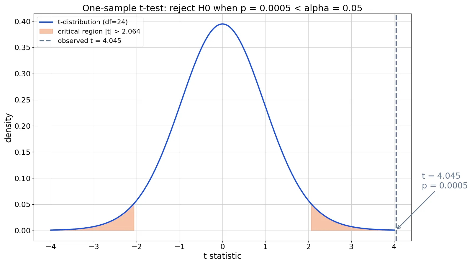
t statistic: $t = (51.3280 - 50.0) / 0.3283 = 4.0450$.
Degrees of freedom: $df = 24$.
Two-sided p-value: $p = 0.0005$.
Critical t at $\alpha = 0.05$: $t_{crit} = 2.0639$.
Decision: $p = 0.0005 < \alpha = 0.05$, so reject $H_0$.

The same result comes from the critical value route. The observed $t = 4.0450$ exceeds $2.0639$ in absolute value, so the test statistic falls in the rejection region.

from scipy import stats
import statistics, math
x = [50.2, 51.8, 49.5, 53.1, 52.4, 48.9, 51.0, 54.2, 50.7, 49.8,
     52.9, 51.3, 50.1, 53.6, 49.2, 52.0, 51.5, 50.4, 53.8, 48.6,
     51.9, 52.7, 50.9, 49.4, 53.3]
t, p = stats.ttest_1samp(x, popmean=50)
print(t, p)  # 4.0450 0.0005

Output:

t = 4.0450, p = 0.0005

The conclusion is that the measurements differ from 50.0 by more than sampling variability alone would explain. The process shows a statistically significant bias at the 0.05 level.

How to Interpret It

A rejected null hypothesis means the data are inconsistent with $H_0$ at your chosen threshold. It does not mean the effect is large or important. Statistical significance measures the size of an effect relative to sampling variability, which is a different question from practical significance [3].

The p-value itself has a narrow meaning. It is the probability of getting a test statistic at least as extreme as the one you observed, assuming $H_0$ is true [1]. It is not the probability that $H_0$ is true, and it is not the probability that your result is a fluke.

When you fail to reject $H_0$, the correct phrasing is that there is insufficient evidence to assert that $H_0$ is false [1]. The test may simply lack power. A small sample or a noisy measurement process can hide a real effect. If you want to understand how the alternative statement shapes the test, see alternative hypothesis.

When to Use It (and when not to)

Use the reject-or-fail-to-reject rule when you have a pre-specified null hypothesis, a test statistic with a known distribution under that null, and a significance level chosen before you look at the data. This covers one-sample and two-sample t-tests, chi-square tests, ANOVA, and most regression coefficient tests.

Do not use it as a substitute for estimation. A confidence interval tells you the range of plausible effect sizes, which is usually more informative than a binary decision. Do not run many tests and report only the significant ones, because that inflates the Type I error rate well above $\alpha$. Do not change $\alpha$ after seeing the p-value, and do not treat $p = 0.049$ and $p = 0.051$ as fundamentally different results.

If your design has confounding or selection problems, no significance threshold will fix them. See avoiding bias in experiments for the design side of this issue.

Rejecting vs Failing to Reject

These two outcomes are not symmetric, and the language reflects that.

Feature	Reject $H_0$	Fail to reject $H_0$
Condition	$p < \alpha$	$p \ge \alpha$
Meaning	Data are unlikely under $H_0$	Insufficient evidence against $H_0$
Error type possible	Type I error	Type II error
Correct phrasing	"The results are statistically significant"	"There is not enough evidence to reject $H_0$"
Incorrect phrasing	"We proved $H_0$ is false"	"We proved $H_0$ is true"

The asymmetry comes from the logic of the test. You assume $H_0$ is true and ask how surprising your data are under that assumption [1]. Failing to reject means the data were not surprising enough, which is not the same as confirming $H_0$.

Common Mistakes

Saying you "accept" the null hypothesis. Failing to reject means the evidence is insufficient, not that $H_0$ is true [1]. Fix: use "fail to reject" or "do not reject" in every write-up.
Treating the p-value as the probability that $H_0$ is true. The p-value is computed conditioned on $H_0$ being true, so it cannot answer that question [1]. Fix: state the p-value as the probability of the data under $H_0$.
Choosing $\alpha$ after seeing the result. This turns a 0.05 test into an arbitrary cutoff. Fix: set $\alpha$ during the design phase and report it.
Confusing statistical and practical significance. A tiny effect can be significant with a large sample [3]. Fix: report an effect size and a confidence interval alongside the p-value.
Ignoring power when you fail to reject. A non-significant result from an underpowered study says little. Fix: report the power or the minimum detectable effect for your design.
Running many tests without adjustment. Each test carries its own Type I error risk, and they compound. Fix: pre-register a primary outcome or apply a multiplicity correction.

Limitations

The reject-or-fail-to-reject rule compresses a continuous measure of evidence into a binary decision. Two studies with p-values of 0.001 and 0.049 both land in the same bucket, even though the evidence differs substantially. The threshold is a convention, not a law of nature, and it says nothing about the size or importance of the effect.

The procedure also depends on assumptions. The t-test used above assumes roughly normal data or a large enough sample for the central limit theorem to apply, and it assumes independent observations. Violating these assumptions can distort the p-value and the rejection decision. For regression settings, check the model assumptions before trusting any coefficient test, as covered in assumptions of linear regression.

Frequently Asked Questions

What does it mean when the null hypothesis is rejected?

It means your sample produced a test statistic extreme enough that the p-value fell below $\alpha$ [1]. In plain language, the data are unlikely if $H_0$ were true. It is evidence against $H_0$, not proof that $H_0$ is false.

Is p = 0.05 enough to reject the null hypothesis?

It depends on your chosen $\alpha$. If $\alpha = 0.05$, then $p = 0.05$ does not meet the strict inequality $p < \alpha$, so you fail to reject [1]. If you set $\alpha = 0.10$ before the study, then $p = 0.05$ would lead to rejection.

Why do we say "fail to reject" instead of "accept"?

Because the test assumes $H_0$ is true from the start and only measures how surprising the data are under that assumption [1]. A non-significant result means the data did not contradict $H_0$, which is weaker than confirming it. The sample may simply be too small or too noisy to detect a real effect.

Can a small p-value occur when the null hypothesis is true?

Yes. A Type I error happens when $H_0$ is true but the test leads you to reject it, and this occurs with probability at most $\alpha$ [3]. With $\alpha = 0.05$, about 5% of tests on true null hypotheses will produce a significant result by chance.

Does rejecting the null hypothesis prove causation?

No. A hypothesis test describes whether an association is larger than sampling variability would explain. Causation requires a design that rules out confounding, such as randomization or careful adjustment. See correlation vs causation for why these are separate questions.

References

Statistical inference
8.1: Why hypothesis testing and Type I and Type II Errors - Statistics LibreTexts/08%3A_Hypothesis_Testing/8.01%3A_Why_hypothesis_testing_and_Type_I_and_Type_II_Errors)
Confidence intervals and hypothesis testing