Assumptions of Linear Regression: Definition and Examples

By Dr. Zubair Khalid, DVM, MS, PhD · 2026-10-03

Linear regression gives you a fitted line, standard errors, p-values and confidence intervals. All of those numbers rest on four assumptions of linear regression analysis: linearity, independence, constant variance and normality of the residuals. If those assumptions fail, the coefficients may still be usable but the inference around them can be wrong.

Quick Answer

Linear regression assumes the mean of the outcome changes in a straight line with each predictor, that observations are independent, that the residual variance is constant, and that residuals are normally distributed [1].
The normality assumption applies to the residuals, not to the predictors or the outcome. Non-normal X and Y are fine as long as the errors are normal [2].
Check linearity and constant variance with a residuals-versus-fitted plot, and normality with a histogram or normal Q-Q plot of the residuals [1].
Formal tests exist for some assumptions. The Breusch-Pagan test checks constant variance, and a small p-value suggests heteroscedasticity.
Most inference methods for regression tolerate mild departures from normality, so plots matter more than pass-or-fail thresholds [1].

What Assumptions of Linear Regression Analysis Means

A plain definition: the assumptions are the conditions under which the fitted line, its standard errors and its p-values behave the way the formulas promise. They describe the data-generating process behind your sample, not the quality of your software.

The precise statistical definition is stated on the model. For a simple regression,

$$y_i = \beta_0 + \beta_1 x_i + \epsilon_i$$

the assumptions are that the errors $\epsilon_i$ have mean zero, constant variance $\sigma^2$, are uncorrelated with each other, and follow a normal distribution. The predictors are treated as fixed. The relationship between the mean of $y$ and $x$ is linear [1].

The same four conditions carry over to multiple regression, where the response has a linear relationship with the predictors in the model [3]. The assumptions of simple regression and the assumptions of multiple regression are the same list, applied to more terms.

How It Works

Each assumption maps to a specific part of the model, and each one protects a specific output.

Linearity. The conditional mean of $y$ is a straight-line function of the predictors. If the true curve bends, the residuals will show a pattern instead of random scatter [1].

Independence. The error for one observation carries no information about the error for another. This matters most with time series, clustered data or repeated measures on the same person.

Constant variance (homoscedasticity). $\text{Var}(\epsilon_i) = \sigma^2$ for every value of $x$. When variance grows with the fitted value, the residuals fan out into a funnel.

Normality of residuals. For a given $x$, the distribution of $y$ around its mean is normal [1]. This is what makes the t and F distributions valid for tests and intervals.

The residual is the raw material for checking all four:

$$\hat{e}_i = y_i - \hat{y}_i$$

where $y_i$ is the observed value and $\hat{y}_i$ is the value the fitted line predicts. A residual is the difference between an observed y-value and the predicted y-value from the regression equation [4]. When the assumptions hold, residuals reflect random chance error only [1].

Worked Example

The dataset below records weekly hours studied and exam scores for 20 students. It is small enough to check by hand and clean enough that the assumptions hold.

hours	score	hours	score
1	52	7	79
2	55	7	81
2	58	8	83
3	60	8	86
3	63	9	88
4	65	9	90
4	68	10	92
5	70	10	94
5	72	11	96
6	74
6	77

The steps follow the least-squares formulas.

Sample size: $n = 20$
Mean hours: $\bar{x} = 120/20 = 6.0000$
Mean score: $\bar{y} = 1503/20 = 75.1500$
Sum of squares: $S_{xx} = 170.0000$
Sum of cross-products: $S_{xy} = 767.0000$
Slope: $b_1 = 767.0000/170.0000 = 4.5118$
Intercept: $b_0 = 75.1500 - 4.5118 \times 6.0000 = 48.0794$
Fitted line: $\hat{y} = 48.0794 + 4.5118 \times \text{hours}$
Residual standard error: $\text{RSE} = \sqrt{36.0265/18} = 1.4147$

The model explains almost all of the variation, with $R^2 = 0.9897$. To test constant variance, the Breusch-Pagan test regresses squared residuals on the predictor. It returns $LM = 0.2030$ with $p = 0.6523$, and an F version of $0.1846$ with $p = 0.6725$. At $\alpha = 0.05$ you fail to reject homoscedasticity, so constant variance is plausible.

import statsmodels.api as sm
from statsmodels.stats.diagnostic import het_breuschpagan
X = sm.add_constant(df['hours'])
model = sm.OLS(df['score'], X).fit()
resid = model.resid
lm, p, f, fp = het_breuschpagan(resid, X)  # BP test for constant variance
print(f"slope={model.params['hours']:.4f}, intercept={model.params['const']:.4f}, R2={model.rsquared:.4f}, RSE={model.mse_resid**0.5:.4f}, BP LM={lm:.4f}, BP p={p:.4f}")

Output:

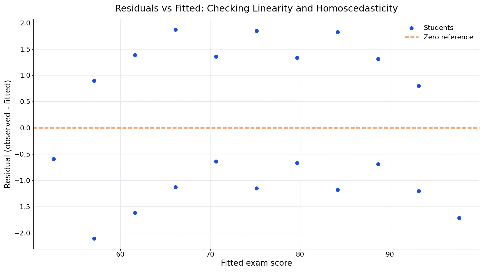
slope=4.5118, intercept=48.0794, R2=0.9897, RSE=1.4147, BP LM=0.2030, BP p=0.6523

A residuals-versus-fitted plot for these 20 students scatters randomly around zero with no funnel shape, which supports both linearity and constant variance. You can reproduce these numbers with a Linear Regression Calculator.

How to Interpret It

Read the diagnostic plots in a fixed order.

Scatterplot of y versus x, before fitting. This is the first check for linearity [1]. A curve here means a straight line is the wrong shape.
Residuals versus fitted values. Look for a horizontal band centered on zero. A U-shape or arch signals missed curvature. A funnel signals changing variance [1].
Residuals versus each predictor. In multiple regression, one predictor can be nonlinear even when the overall plot looks fine [3].
Histogram and normal Q-Q plot of residuals. Points close to the diagonal line on the Q-Q plot support normality [1]. Heavy tails or strong skew point the other way.
Residuals versus observation number. Use this when the data have a natural order, such as time. A wave or drift suggests dependence between observations [3].

For the exam data, all five checks are clean. The slope of 4.5118 means each extra hour of study is associated with about 4.5 more points on the exam, and the Breusch-Pagan p-value of 0.6523 is well above 0.05.

When to Use It (and when not to)

Use linear regression when the outcome is continuous, the relationship is roughly straight, and observations can be treated as independent. It is the right default for prediction and for estimating adjusted associations in observational data, and it extends naturally to multiple linear regression with confounders and interactions.

Do not force it when the outcome is a count, a proportion or a binary flag. Those need a different error distribution, which is what generalized linear models provide. Do not use ordinary least squares when the relationship is clearly curved and you have not modeled the curve, for example with a quadratic term. Do not ignore clustering. If students are nested in classrooms, standard errors from ordinary least squares will be too small.

Assumptions vs Diagnostics

The assumptions are properties of the population. Diagnostics are what you compute on the sample to judge them. Keeping the two apart prevents a common confusion.

Item	Assumptions	Diagnostics
What it is	Conditions on the error term	Sample-based evidence about those conditions
Linearity	Mean of y is linear in x	Scatterplot, residuals vs fitted
Constant variance	$\text{Var}(\epsilon) = \sigma^2$	Residual funnel plot, Breusch-Pagan test
Normality	Errors are normal	Histogram, normal Q-Q plot
Independence	Errors are uncorrelated	Residuals vs observation order, study design
Can it be proven?	No	No, only supported or contradicted

Common Mistakes

Testing normality of the outcome instead of the residuals. The assumption is about residuals [2]. Fix: run the histogram and Q-Q plot on the residuals from the fitted model.
Treating a non-significant test as proof the assumption holds. A Breusch-Pagan p-value of 0.6523 means the data are consistent with constant variance, not that variance is exactly equal. Fix: read the plot alongside the test.
Ignoring a funnel because the p-value looks fine. Tests lose power in small samples. Fix: with n = 20, trust the shape of the residual plot over the test.
Checking linearity after fitting and stopping there. The scatterplot of y versus x should be inspected before the model is fit [1]. Fix: plot the raw data first.
Assuming independence because the data look tidy. Independence comes from the study design, not from the file layout. Fix: ask how the observations were collected and whether any are linked.
Dropping outliers to make plots look better. An outlier may be the most informative point. Fix: investigate it, and report any removal.

Limitations

Diagnostics cannot prove that assumptions hold. They can only show patterns that are hard to reconcile with them, and small samples make every plot noisy. A clean residual plot in a study of 20 students is weak evidence compared with the same plot in a study of 2,000.

The tests have their own limits. Breusch-Pagan detects certain forms of changing variance and can miss others. Normality tests are sensitive in large samples, where trivial departures become significant, and underpowered in small ones. The assumptions also say nothing about whether your model includes the right predictors, whether the sample represents the population you care about, or whether a relationship is causal. A model can satisfy every assumption and still answer the wrong question.

Frequently Asked Questions

What are the four main assumptions of linear regression analysis?

Linearity, independence of observations, constant variance of the residuals, and normality of the residuals [1]. Some texts list a fifth, that the predictors are measured without error or are fixed by design. Together these conditions make the standard errors, t tests and confidence intervals valid.

Do the predictors and outcome need to be normally distributed?

No. The normality assumption applies to the residuals, and it is acceptable for the predictors and the outcome to be non-normal as long as the residuals are normal [2]. This is one of the most commonly misunderstood points in regression.

How do I check the linearity assumption in multiple regression?

Plot residuals against fitted values and against each predictor separately [3]. A random cloud around zero supports linearity. A curve, arch or systematic band means the model is missing curvature or an interaction, and you should add the relevant term.

What should I do if the constant variance assumption fails?

First confirm the pattern in the residual plot. Then consider a transformation of the outcome, such as a log or square root, or use a model that allows the variance to change with the mean. Weighted least squares and heteroscedasticity-consistent standard errors are common alternatives.

Can I still use my regression if an assumption is violated?

Often yes, with care. Mild departures from normality usually leave inference roughly intact [1], and the coefficient estimates themselves stay unbiased under several violations. The risk is concentrated in the standard errors and p-values, so report the diagnostics and use a method suited to the problem.