What Is Hypothesis Testing? Steps, Errors and Examples

By Dr. Zubair Khalid, DVM, MS, PhD · 2026-10-03

Hypothesis testing is a decision-making procedure that uses sample data to judge whether a claim about a population is supported. You state two competing claims, measure how far your sample result falls from the claim, and decide whether that distance is large enough to be meaningful. This article walks through the logic, the steps, the two error types, and a complete worked example.

Quick Answer

Hypothesis testing compares two statements: a null hypothesis ($H_0$) of "no difference" and an alternative hypothesis ($H_a$) of a real difference [1].
You compute a test statistic from your sample, then compare it to a distribution that assumes $H_0$ is true [2].
The p-value is the probability of seeing a result at least as extreme as yours if $H_0$ were true. A small p-value is evidence against $H_0$ [3].
Two errors are possible: rejecting a true $H_0$ (Type I, probability $\alpha$) and failing to reject a false $H_0$ (Type II, probability $\beta$) [1].
A test never proves $H_0$ true. It only tells you whether the data are consistent with it [4].

What Hypothesis Testing Means

In plain terms, hypothesis testing is the process of making a choice between two conflicting hypotheses using data [1]. You start with a question like "Is the average satisfaction score different from 7?" and end with a decision: reject the null hypothesis or fail to reject it.

The precise statistical definition is narrower. A statistical hypothesis is a statement about a population parameter, such as a mean, proportion, or variance. The null hypothesis ($H_0$) states that there is no significant difference between a hypothesized value of a population parameter and its value estimated from a sample [1]. The alternative hypothesis ($H_1$ or $H_a$) states that a significant difference exists [1].

The test procedure is built so that the risk of rejecting $H_0$ when it is actually true stays small [4]. That controlled risk is what makes the decision defensible. If you want more detail on writing these statements, see null and alternative hypotheses.

How It Works

Every test follows the same mechanism. You assume $H_0$ is true, then ask how surprising your sample would be under that assumption.

The general test statistic has this form:

$$t = \frac{\bar{x} - \mu_0}{SE}$$

Each symbol means:

$\bar{x}$ is the sample mean, your observed average.
$\mu_0$ is the hypothesized population mean under $H_0$.
$SE$ is the standard error, computed as $s / \sqrt{n}$, where $s$ is the sample standard deviation and $n$ is the sample size.
$t$ is the number of standard errors your sample mean sits away from the hypothesized value.

Once you have $t$, you compare it to a reference distribution. For a one-sample t-test, that is the t-distribution with $n - 1$ degrees of freedom. The p-value is the proportion of that distribution as extreme as, or more extreme than, your observed statistic [2]. If the p-value falls below your chosen $\alpha$, you reject $H_0$.

Worked Example

A company surveys 15 customers on a 1 to 10 satisfaction scale and wants to know whether the average score differs from a benchmark of 7.0. The raw scores are below.

Customer	Score
1	8
2	7
3	9
4	6
5	8
6	7
7	8
8	9
9	7
10	6
11	8
12	7
13	9
14	8
15	7

The hypotheses are $H_0: \mu = 7.0$ and $H_a: \mu \neq 7.0$, tested at $\alpha = 0.05$.

Step by step:

Sample size: $n = 15$.
Sample mean: $\bar{x} = 7.6000$.
Sample standard deviation: $s = 0.9856$.
Standard error: $SE = s / \sqrt{n} = 0.9856 / \sqrt{15} = 0.2545$.
Test statistic: $t = (7.6000 - 7.0) / 0.2545 = 2.3577$.
Degrees of freedom: $df = n - 1 = 14$.
Critical value: $t_{crit} = 2.1448$ for a two-tailed test at $\alpha = 0.05$.
p-value: $p = 0.0335$.
Decision: since $|t| = 2.3577 > t_{crit} = 2.1448$, reject $H_0$.

Here is the same test in Python:

from scipy import stats
scores = [8,7,9,6,8,7,8,9,7,6,8,7,9,8,7]
t, p = stats.ttest_1samp(scores, popmean=7.0)
print(t, p)  # 2.3577 0.0335

Output:

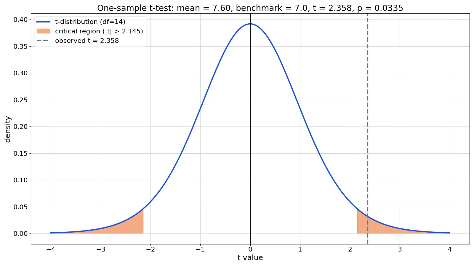
t = 2.3577, p = 0.0335

The observed t of 2.3577 sits beyond the critical value of 2.1448, so it lands in the rejection region. The p-value of 0.0335 means that if the true mean were exactly 7.0, you would see a t statistic at least this far from 0, in either direction, about 3.35% of the time. That is below 0.05, so the data provide evidence against the null hypothesis.

How to Interpret It

The p-value measures the consistency between the null hypothesis and the observed test statistic, and it should be interpreted carefully [2]. A small p-value means your data are unlikely under $H_0$. It does not mean $H_0$ is false with probability $p$, and it does not measure the size of the effect.

Two decisions are possible, and each can be right or wrong [1]:

Reality	You reject $H_0$	You fail to reject $H_0$
$H_0$ is true	Type I error ($\alpha$)	Correct decision
$H_0$ is false	Correct decision	Type II error ($\beta$)

A Type I error means you rejected a true null hypothesis. Its probability is $\alpha$, which you set in advance, commonly at 0.05 [1]. A Type II error means you failed to reject a false null hypothesis, with probability $\beta$ [1]. The quantity $1 - \beta$ is called power.

In the worked example, rejecting $H_0$ could be a Type I error if the true mean really is 7.0. You accepted a 5% chance of that mistake when you set $\alpha = 0.05$. For more on the decision rule itself, see when to reject the null hypothesis.

When to Use It (and when not to)

Use hypothesis testing when you have a specific claim about a population parameter and sample data that can address it. It fits controlled experiments, survey comparisons, quality checks, and clinical trials. Most medical and epidemiological studies are designed around a hypothesis test, which is why reading them well depends on understanding the key principles [3].

Do not use it when you have no prior claim to test. If you are exploring data for patterns, a confidence interval or a descriptive summary is more honest than running many tests and reporting the ones that came out significant. Multiple tests inflate your error rate, a problem that grows with every additional comparison [3].

Also avoid it when your sample is too small to detect an effect you care about. A non-significant result from an underpowered study is uninformative, because it cannot distinguish "no effect" from "not enough data" [4].

Hypothesis Testing vs Confidence Intervals

Both are classical methods for generalizing from a sample to a population [2]. They answer related questions from different angles.

Feature	Hypothesis Test	Confidence Interval
Question answered	Is there evidence against a specific value?	What range of values is plausible?
Output	Test statistic and p-value	Interval with a confidence level
Decision	Reject or fail to reject $H_0$	No formal reject or fail decision
Effect size	Not shown directly	Shown by the interval width and center
Best for	Testing a stated claim	Estimating a parameter

A 95% confidence interval and a two-tailed test at $\alpha = 0.05$ often agree. If the interval excludes the null value, the test typically rejects $H_0$. The interval adds information the p-value hides: how large the effect might be.

Common Mistakes

Interpreting the p-value as the probability that $H_0$ is true. The p-value is computed assuming $H_0$ is true, so it cannot be the probability of $H_0$ [3]. Fix: describe it as the probability of the data given $H_0$, not the reverse.
Treating "fail to reject" as "accept $H_0$." Not rejecting means the data are consistent with $H_0$, not that $H_0$ is proven [4]. Fix: report the confidence interval alongside the test.
Confusing statistical significance with practical importance. A tiny effect can be significant with a large sample. Fix: report the effect size and its units.
Running many tests and reporting only the significant ones. Each test carries its own Type I error risk, so the family-wise error rate climbs [3]. Fix: pre-specify your primary test or apply a correction.
Choosing $\alpha$ after seeing the p-value. This turns a controlled decision into a rationalization. Fix: set $\alpha$ before collecting data.
Ignoring power when planning. Low power makes Type II errors likely and non-significant results hard to read [5]. Fix: run a power calculation during study design.

Limitations

A hypothesis test cannot prove a hypothesis true. It can only tell you whether the observed data are unusual under a specified null model [4]. A non-significant result may reflect a true null, a small effect, a noisy measurement, or simply too little data.

The framework also reduces a rich result to a binary decision. The p-value depends on sample size, so the same effect can be significant in one study and not in another. It says nothing about bias, confounding, or study design quality. A well-executed test on a badly designed study still produces a misleading answer. For questions about cause, remember that a significant test does not establish causation, as covered in correlation vs causation.

Frequently Asked Questions

What is the difference between a null and alternative hypothesis?

The null hypothesis states there is no significant difference between a hypothesized population parameter value and its sample estimate [1]. The alternative hypothesis states that a significant difference exists [1]. They are mutually exclusive, and the test decides between them. See alternative hypothesis for how to write the second one.

What does a p-value of 0.03 actually mean?

It means that if the null hypothesis were true, you would observe a test statistic at least as extreme as yours about 3% of the time [2]. It is a statement about the data under $H_0$, not about the probability that $H_0$ is correct. A common threshold is 0.05, but the right cutoff depends on the cost of each error type.

What is the difference between Type I and Type II errors?

A Type I error is rejecting the null hypothesis when it is true, with probability $\alpha$ [1]. A Type II error is failing to reject the null hypothesis when it is false, with probability $\beta$ [1]. Lowering $\alpha$ reduces Type I errors but usually increases Type II errors unless you increase sample size.

Can I use hypothesis testing with a small sample?

Yes, but the test must match the data. The one-sample t-test in the worked example uses the t-distribution, which accounts for the extra uncertainty of a small sample through its degrees of freedom. With very small samples, power is low, so a non-significant result is weak evidence either way [5].

Does a significant result mean the effect is large?

No. Significance depends on both the effect size and the sample size. A very small difference can produce a small p-value when $n$ is large. Always report the effect size and a confidence interval so readers can judge practical importance. If you are comparing two groups, the two sample t-test shows how the same logic extends.

References

- Yarandi HN. (1996). Hypothesis testing. Clinical nurse specialist CNS
- Hypothesis Testing - Stat 20
- Pugh SL, Molinaro A. (2016). The nuts and bolts of hypothesis testing. Neuro-oncology practice
- 7.1.3. What are statistical tests?
- Ranganathan P, Cs P. (2019). An Introduction to Statistics: Understanding Hypothesis Testing and Statistical Errors. Indian journal of critical care medicine : peer-reviewed, official publication of Indian Society of Critical Care Medicine
Further Reading
- 3.1: The Fundamentals of Hypothesis Testing - Statistics LibreTexts/03%3A_Hypothesis_Testing/3.01%3A_The_Fundamentals_of_Hypothesis_Testing)
- 6.5 Introduction to Hypothesis Tests - Significant Statistics - beta (extended) version
Related Articles
- Alternative Hypothesis: Definition, Examples and How to Write It
- When to Reject the Null Hypothesis: Definition and Examples
- Null and Alternative Hypotheses: Definition and Examples
- Simple Random Sampling: Definition, Steps and Examples
- Dependent Variable Examples: Definition and Study Design
- How to Write a Hypothesis for a Research Proposal: Examples and Templates
- Bayesian Hypothesis Testing for Biological Data
- How to Write a Hypothesis for an Experimental Study