t Statistic Formula: Definition, Calculation and Examples

By Dr. Zubair Khalid, DVM, MS, PhD · 2026-10-03

The t statistic formula measures how many standard errors a sample mean lies from a hypothesized value. You use it when the population standard deviation is unknown and you estimate it from your sample. This article gives the exact formula, explains every symbol, and works through a full calculation.

Quick Answer

The t statistic formula is $t = \dfrac{\bar{x} - \mu}{s / \sqrt{n}}$.
$\bar{x}$ is the sample mean, $\mu$ is the hypothesized population mean, $s$ is the sample standard deviation, and $n$ is the sample size.
The denominator $s / \sqrt{n}$ is the standard error of the mean.
The degrees of freedom for a one-sample test are $df = n - 1$.
A larger absolute t value means the sample mean is farther from $\mu$ in standard error units, which is evidence against the null hypothesis.

The Formula

For a one-sample t-test, the t statistic formula is:

$$t = \frac{\bar{x} - \mu}{s / \sqrt{n}}$$

Each symbol has a specific job:

Symbol	Meaning
$\bar{x}$	Sample mean, the average of your observed values
$\mu$	Hypothesized population mean, the value in the null hypothesis
$s$	Sample standard deviation, computed with $n - 1$ in the denominator
$n$	Number of observations in the sample
$s / \sqrt{n}$	Standard error of the mean (SE)
$df$	Degrees of freedom, $n - 1$ for a one-sample test

The numerator $\bar{x} - \mu$ is the raw distance between your estimate and the hypothesized value. Dividing by the standard error rescales that distance into units of sampling variability. That is why t is often called a signal-to-noise ratio: the signal is the difference in means, and the noise is the standard error.

The same structure appears in other t tests. For two independent groups, the numerator becomes the difference in sample means and the denominator becomes the standard error of that difference. The two sample t-test formula and example covers that case, including the pooled and Welch versions.

How to Calculate It Step by Step

State the null hypothesis value $\mu$. This is the benchmark you are testing against, such as a target, a historical average, or a specification.
Count your observations to get $n$.
Compute the sample mean $\bar{x}$ by adding all values and dividing by $n$. If you need a refresher, the sample mean guide walks through the arithmetic.
Compute the sample standard deviation $s$ using $n - 1$ in the denominator. This is the sample SD, not the population SD.
Compute the standard error: $SE = s / \sqrt{n}$.
Compute the numerator: $\bar{x} - \mu$.
Divide the numerator by the standard error to get $t$.
Set the degrees of freedom: $df = n - 1$.
Compare your t value against a t distribution with those degrees of freedom. The Student's t-distribution guide explains the shape and why df matters.

Worked Example

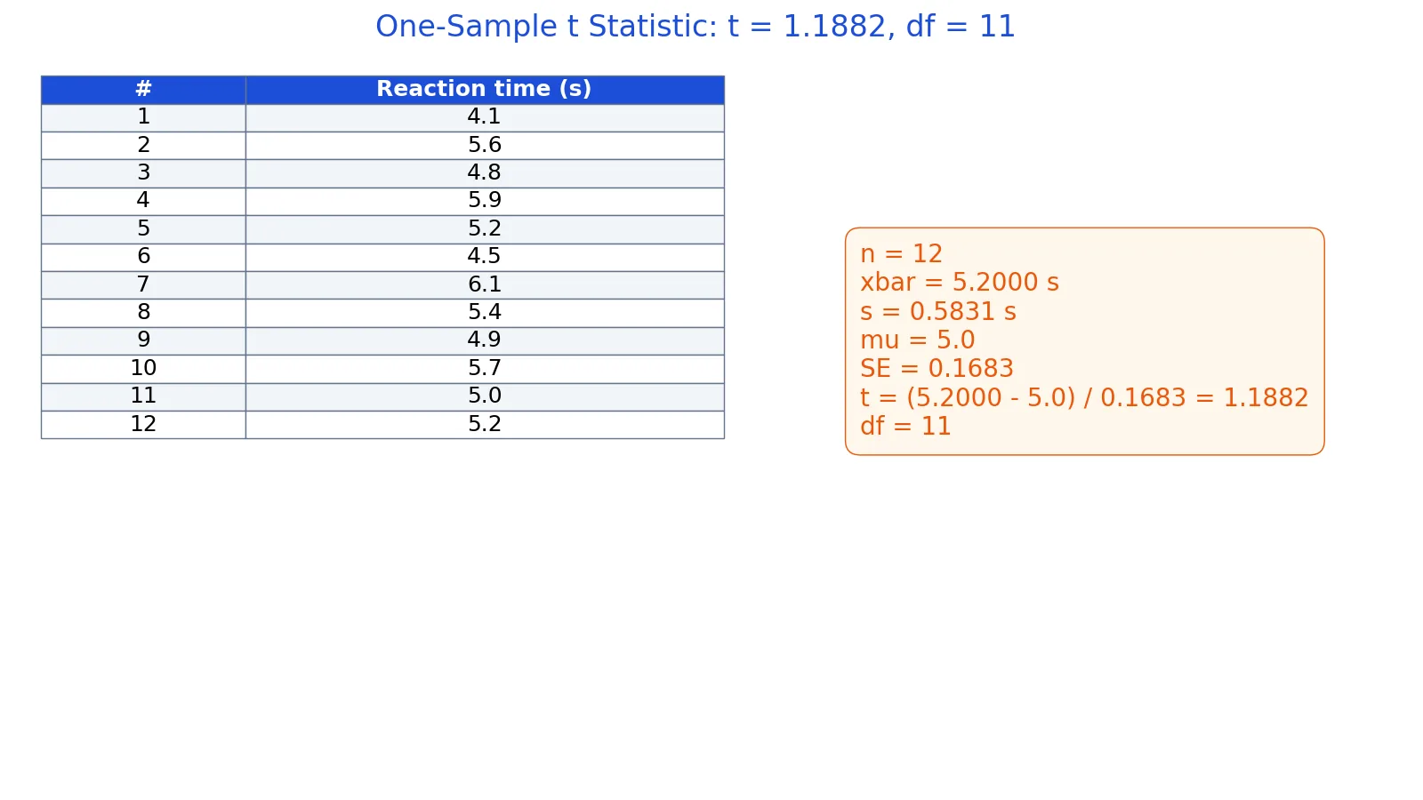
A lab records reaction times in seconds across 12 trials. The team wants to know whether the mean reaction time differs from a benchmark of 5.0 seconds.

trial	reaction_time_s
1	4.1
2	5.6
3	4.8
4	5.9
5	5.2
6	4.5
7	6.1
8	5.4
9	4.9
10	5.7
11	5.0
12	5.2

Step 1. Sample size: $n = 12$.

Step 2. Sample mean: the values sum to 62.4, so $\bar{x} = 62.4 / 12 = 5.2000$.

Step 3. Sample standard deviation: $s = 0.5831$.

Step 4. Standard error: $SE = s / \sqrt{n} = 0.5831 / \sqrt{12} = 0.1683$.

Step 5. t statistic: $t = (\bar{x} - \mu) / SE = (5.2000 - 5.0) / 0.1683 = 1.1882$.

Step 6. Degrees of freedom: $df = n - 1 = 12 - 1 = 11$.

The result is $t = 1.1882$ with $df = 11$. The sample mean sits about 1.19 standard errors above the benchmark.

Here is the same calculation in Python:

import statistics, math
times = [4.1, 5.6, 4.8, 5.9, 5.2, 4.5, 6.1, 5.4, 4.9, 5.7, 5.0, 5.2]
n = len(times)
xbar = statistics.mean(times)
s = statistics.stdev(times)
mu = 5.0
t = (xbar - mu) / (s / math.sqrt(n))
df = n - 1
print(t, df)  # prints 1.1882... and 11

Output: t = 1.1882, df = 11.

How to Interpret the Result

The t value alone does not tell you whether the difference is statistically significant. You need the degrees of freedom and a decision rule.

For a two-sided test at the 0.05 level with $df = 11$, you compare your t value to a critical value from the t table. If the absolute t value exceeds the critical value, you reject the null hypothesis. If it does not, you fail to reject.

You can also convert t to a p-value directly. The t to p-value guide shows how the conversion works and what the resulting probability means. For the example above, the p-value is larger than 0.05, so the observed mean of 5.2000 seconds is consistent with a true mean of 5.0 seconds at that significance level.

Three things shape the size of t:

A bigger difference $\bar{x} - \mu$ pushes t away from zero.
A smaller standard deviation shrinks the standard error and pushes t away from zero.
A larger sample size shrinks the standard error through $\sqrt{n}$ and also pushes t away from zero.

That last point is why a small difference can still produce a large t when the sample is large.

Doing It in Software

You rarely compute t by hand for real work. These functions handle the arithmetic and the p-value.

Excel. T.TEST returns the p-value for a t-test. Its arguments are the two data ranges, the number of tails, and the test type. For a one-sample test against a constant, you can compute t manually with AVERAGE, STDEV.S, COUNT, and SQRT, then use T.DIST.2T to get the two-tailed p-value from the absolute t value and the degrees of freedom.

R. The t.test function performs one and two sample t-tests on vectors of data [1]. By default, if var.equal is FALSE, the variance is estimated separately for both groups and the Welch modification to the degrees of freedom is used [1]. The mu argument sets the true value of the mean, or the difference in means for a two-sample test [1]. The returned object includes the degrees of freedom for the t-statistic and a confidence interval for the mean [1].

Python. The scipy.stats.ttest_1samp function takes your data array and the hypothesized mean, and returns the t statistic and p-value. The snippet in the worked example shows the manual route if you want to see each piece.

If you want to skip the manual steps, the T-Test Calculator takes your data and returns the t statistic, degrees of freedom, and p-value.

Common Mistakes

Using the population SD instead of the sample SD. The t statistic requires $s$ computed with $n - 1$ in the denominator. Using a known population $\sigma$ calls for a z statistic instead.
Forgetting to divide by $\sqrt{n}$. The denominator is the standard error, not the standard deviation. Dividing by $s$ alone gives a number that grows with sample size for no good reason.
Reporting t without degrees of freedom. A t value of 2.0 means different things at $df = 5$ and $df = 500$. Always report both.
Mixing up one-tailed and two-tailed p-values. Decide the direction of your test before you look at the data. Halving a two-tailed p-value after seeing the direction of the data is a form of p-hacking.
Treating a large t as proof of a large effect. With a big enough sample, a trivial difference can produce a large t. Report the effect size and a confidence interval alongside the test.
Ignoring the assumptions. The one-sample t-test assumes independent observations and an approximately normal sampling distribution. Check for outliers and clustering before you trust the result.

Limitations

The t statistic formula assumes your observations are independent and that the sample mean is approximately normally distributed. With small samples, that normality assumption matters more. If your data are heavily skewed or contain extreme outliers, the t test can mislead you. R notes that wilcox.test is robust against outliers and deals more usefully with infinite values in the data [1].

The test also answers a narrow question. It tells you whether the mean differs from a hypothesized value, not whether the difference is practically meaningful. A significant result with a tiny effect size may have no consequence for your decision. And the t statistic says nothing about the shape of the distribution, the presence of subgroups, or whether your sample represents the population you care about. Those are design questions the formula cannot answer.

Frequently Asked Questions

What is the difference between the t statistic and the t value?

They are the same thing. "t statistic," "t value," "t score," and "t stat" all refer to the number produced by the formula. The term "t statistics formula" is just a plural phrasing of the same calculation.

What is the formula for the t statistic in a two-sample test?

For two independent groups, the numerator becomes $\bar{x}_1 - \bar{x}_2$ and the denominator becomes the standard error of that difference. The exact denominator depends on whether you assume equal variances. R uses the Welch approximation by default when var.equal is FALSE [1].

How do I find the degrees of freedom?

For a one-sample t-test, $df = n - 1$. For a paired test, $df$ equals the number of pairs minus one. For a two-sample test with equal variances, $df = n_1 + n_2 - 2$. The Welch version uses a more complex approximation that usually produces a non-integer value [1].

Can the t statistic be negative?

Yes. A negative t means the sample mean is below the hypothesized value. For a two-sided test, you compare the absolute value of t to the critical value. The sign still carries information about direction.

What sample size do I need for the t statistic to be valid?

There is no fixed cutoff. The t distribution accounts for small samples through the degrees of freedom. What matters more is whether the data are independent and roughly symmetric. With very small samples, a single outlier can dominate the result, so inspect the data before trusting the number.

References

R: Student's t-Test

References

Further Reading
- Krzywinski M, Altman N (2013). Significance, P values and t-tests. Nature Methods
- NIST/SEMATECH e-Handbook of Statistical Methods
- Wasserstein RL, Lazar NA (2016). The ASA Statement on p -Values: Context, Process, and Purpose. The American Statistician
- OpenStax. Introductory Statistics 2e
- Krzywinski M, Altman N (2013). Importance of being uncertain. Nature Methods
Related Articles
- Student's t-Distribution: Definition, Formula and Examples
- Two Sample t-Test: Formula, Calculation and Example
- Formula for Range: Definition, Formula and Examples
- Covariance Formula: Definition and Calculation Examples
- T to P-Value: Convert a t Statistic to a P-Value
- Test Statistic Formula: How to Calculate and Use It
- One-Sample t-Test: Formula, Calculation, and Interpretation
- Understanding the t-Test Table: How to Use It for Significance