Frequency Distribution: Definition, Table and Examples
By Dr. Zubair Khalid, DVM, MS, PhD ·
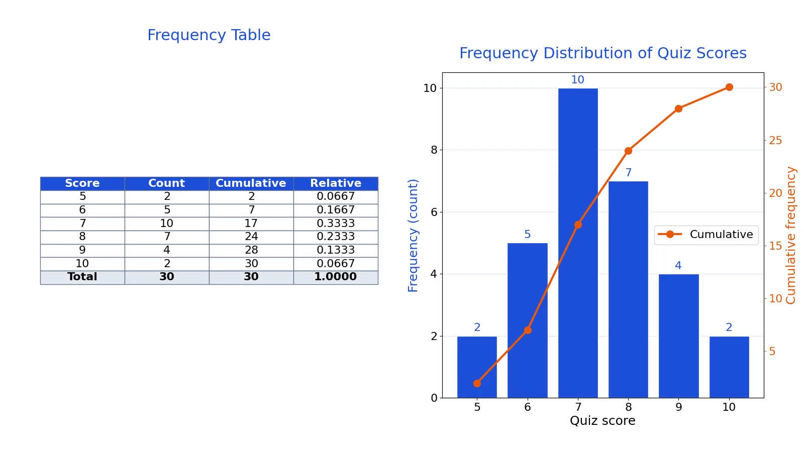
A frequency distribution is a summary that lists each value or group of values in a dataset and how often it occurs. It turns a long list of raw numbers into a compact table you can read at a glance. This article defines the term, shows the formulas for frequency, cumulative frequency and relative frequency, and builds a full frequency table from 30 quiz scores.
Quick Answer
- A frequency distribution lists every data value (or class) and its frequency, which is the number of times that value appears [1].
- Frequency answers "how many?" for each value. You find it by counting how many times each value occurs in the raw data.
- A frequency table has at least two columns: the values (X) and their frequencies (f) [2].
- Cumulative frequency adds each row's frequency to the running total of all previous rows [3].
- Relative frequency is the frequency divided by the sample size $n$, giving the proportion of the dataset in each value or class [1].
What Frequency Distribution Means
In plain terms, a frequency distribution is a count of how many times each value shows up in your data. If five students scored 6 on a quiz, then 6 has a frequency of 5.
The precise statistical definition: a frequency distribution is an organized tabulation showing exactly how many individuals or units of measurement fall into each category on the scale of measurement [2]. It contains the entire set of scores and lets you compare each score to the rest of the set.
The word "frequency" itself means the number of times a data value, or a group of data values called classes, occurs in a dataset [1]. When values are grouped into ranges, those ranges are the classes, and the table is called a grouped frequency distribution. When every distinct value gets its own row, it is an ungrouped frequency distribution.
How It Works
Building a frequency distribution comes down to counting. For each distinct value in your data, count how many observations equal that value. That count is the frequency.
Three formulas cover almost everything you will need.
Frequency. For each value $x_i$, the frequency $f_i$ is the number of observations equal to $x_i$. The frequencies must sum to the sample size:
$$\sum_{i=1}^{k} f_i = n$$
where $k$ is the number of distinct values or classes, $f_i$ is the frequency of the $i$-th value, and $n$ is the total number of observations.
Cumulative frequency. The cumulative frequency for a row is the sum of that row's frequency and all frequencies above it [3]:
$$\text{cum}_i = \text{cum}_{i-1} + f_i$$
The last cumulative value always equals $n$, because it has accumulated every observation in the dataset.
Relative frequency. The relative frequency is the frequency divided by the sample size [1]:
$$\text{rel}_i = \frac{f_i}{n}$$
Relative frequencies are proportions between 0 and 1, and they sum to 1 (up to rounding) [2]. Multiply by 100 to express them as percentages.
Worked Example
The dataset is the quiz scores (out of 10) of 30 students. Here are the raw values, one row per student.
| Student | Score | Student | Score | Student | Score |
|---|---|---|---|---|---|
| 1 | 7 | 11 | 8 | 21 | 6 |
| 2 | 8 | 12 | 7 | 22 | 7 |
| 3 | 6 | 13 | 9 | 23 | 10 |
| 4 | 9 | 14 | 6 | 24 | 8 |
| 5 | 7 | 15 | 7 | 25 | 7 |
| 6 | 5 | 16 | 8 | 26 | 6 |
| 7 | 8 | 17 | 5 | 27 | 9 |
| 8 | 7 | 18 | 9 | 28 | 7 |
| 9 | 10 | 19 | 7 | 29 | 8 |
| 10 | 6 | 20 | 8 | 30 | 7 |
Step 1: Count the observations. There are $n = 30$ scores.
Step 2: List the distinct values. The scores that appear are 5, 6, 7, 8, 9 and 10.
Step 3: Count each value. Score 5 appears 2 times, score 6 appears 5 times, score 7 appears 10 times, score 8 appears 7 times, score 9 appears 4 times, and score 10 appears 2 times.
Step 4: Build the cumulative column. Start with 2 for score 5. Add 5 to get 7 for score 6. Add 10 to get 17 for score 7. Add 7 to get 24 for score 8. Add 4 to get 28 for score 9. Add 2 to get 30 for score 10, which matches $n$.
Step 5: Compute relative frequencies. Divide each count by 30. Score 5 gives $2/30 = 0.0667$, score 6 gives $5/30 = 0.1667$, score 7 gives $10/30 = 0.3333$, score 8 gives $7/30 = 0.2333$, score 9 gives $4/30 = 0.1333$, and score 10 gives $2/30 = 0.0667$.
The finished table:
| Score | Frequency | Cumulative frequency | Relative frequency | Cumulative relative frequency |
|---|---|---|---|---|
| 5 | 2 | 2 | 0.0667 | 0.0667 |
| 6 | 5 | 7 | 0.1667 | 0.2333 |
| 7 | 10 | 17 | 0.3333 | 0.5667 |
| 8 | 7 | 24 | 0.2333 | 0.8000 |
| 9 | 4 | 28 | 0.1333 | 0.9333 |
| 10 | 2 | 30 | 0.0667 | 1.0000 |
The same table in Python:
import pandas as pd
scores = [7, 8, 6, 9, 7, 5, 8, 7, 10, 6,
          8, 7, 9, 6, 7, 8, 5, 9, 7, 8,
          6, 7, 10, 8, 7, 6, 9, 7, 8, 7]
s = pd.Series(scores)
freq = s.value_counts().sort_index()
table = pd.DataFrame({'count': freq,
                      'cumulative': freq.cumsum(),
                      'relative': (freq / freq.sum()).round(4)})
print(table)
Output:
    count  cumulative  relative
5       2           2    0.0667
6       5           7    0.1667
7      10          17    0.3333
8       7          24    0.2333
9       4          28    0.1333
10      2          30    0.0667
How to Interpret It
Read the frequency column first. The largest count is the mode, the most common value. Here the mode is 7, with 10 students out of 30. The smallest count tells you which value is rarest, and if a value has a frequency of 0 it should still appear in the table so the gap is visible [4].
The cumulative column answers "how many at or below this value?" A cumulative frequency of 17 at score 7 means 17 students scored 7 or lower. The final cumulative value always equals the sample size, which is a quick check that you counted everything.
The relative frequency column answers "what share?" A relative frequency of 0.3333 for score 7 means one third of the class scored 7. The cumulative relative frequency of 0.8000 at score 8 means 80 percent of students scored 8 or below. The last entry should be 1.00, or close to it after rounding [3].
For this dataset, the mean is 7.4, the median is 7 and the mode is 7. The frequency table makes the mode obvious without any calculation.
When to Use It (and when not to)
Use a frequency distribution when you first receive a dataset and want a quick picture of its shape. It works well for categorical data such as favorite colors or vehicle makes, where you simply count each category [1][5]. It also works for discrete numeric data with a modest number of distinct values, such as quiz scores, number of children, or ratings on a 1 to 5 scale.
Use a grouped frequency distribution when a numeric variable has many distinct values, such as salaries or heights. You split the range into class intervals and count how many observations fall in each one [6]. Class intervals should be mutually exclusive and nonoverlapping, and open-ended classes such as "under 10" or "over 100" should be avoided [6].
Do not use a frequency distribution when you need to preserve every individual value for further calculation, such as computing a regression. The table summarizes and discards the raw values. For very large datasets with continuous measurements, a histogram or frequency polygon communicates the same information more efficiently than a long table [5][6].
Frequency Distribution vs Frequency Table
The two terms are closely related but not identical. A frequency distribution is the concept, the pairing of values with their counts. A frequency table is the physical layout that displays that pairing in rows and columns [2]. Every frequency table represents a frequency distribution, but you can also describe a frequency distribution in words or show it as a graph.
| Feature | Frequency distribution | Frequency table |
|---|---|---|
| What it is | The pairing of values or classes with their frequencies | The tabular layout that displays the pairing |
| Form | Concept, can be described in words or shown as a graph | Rows and columns with labeled headers |
| Minimum content | Values and their counts | At least an X column and an f column [2] |
| Extra columns | Can include relative or cumulative frequency | Often adds cumulative and relative columns [3] |
| Typical use | Describing the shape of a dataset | Presenting the counts to a reader |
If you want a deeper walkthrough of the table format itself, see Frequency Table: Definition, How to Make One, Examples.
Common Mistakes
- Skipping values with a frequency of 0. If no one scored 4, leave the row for 4 in the table with a count of 0. Omitting it hides the gap and makes the table harder to trust [4]. Fix: list every value in the range, even empty ones.
- Letting class intervals overlap. Intervals like 10 to 20 and 20 to 30 double-count the boundary value. Fix: make intervals mutually exclusive, for example 10 to 19 and 20 to 29 [6].
- Forgetting to check the total. The frequency column must sum to $n$. If it does not, you miscounted. Fix: add the column and compare it to the number of observations.
- Confusing frequency with relative frequency. A count of 10 and a proportion of 0.3333 describe the same row but mean different things. Fix: label the columns clearly and check that relative frequencies sum to 1 [1].
- Adding rounded relative frequencies to get cumulative values. Rounding errors accumulate. Fix: compute each cumulative relative frequency from the cumulative count divided by $n$, then round [4].
- Using too many or too few classes. Too many classes produce a sparse table, too few hide the shape. Fix: aim for a small number of intervals that each contain several observations.
Limitations
A frequency distribution summarizes counts, not magnitudes. Two datasets with identical frequency tables can have very different means if the underlying values differ, so the table alone cannot tell you the average or the spread. It also discards the identity of individual observations, which means you cannot recover the raw data or link scores back to specific students once the table is built.
For continuous data, the result depends heavily on how you define the class intervals. Shifting the boundaries can change which interval a value falls into and alter the apparent shape of the distribution. Frequency tables also become unwieldy when a variable has hundreds of distinct values, and at that point a graph or a summary statistic serves you better [6].
Frequently Asked Questions
How do you calculate frequency?
Count how many times each value appears in the dataset. If the value 7 appears 10 times, its frequency is 10. In a spreadsheet you can use a count function, and in Python you can use value_counts() on a pandas Series, as shown in the worked example above.
What is the difference between frequency and cumulative frequency?
Frequency is the count for one value or class on its own. Cumulative frequency is the running total, adding each row's frequency to all the rows before it [3]. The final cumulative frequency always equals the total number of observations.
How do you find the class with the least number of data values?
Look down the frequency column and find the smallest count. That row's class is the one with the least data values. If several classes tie for the smallest count, they all share that distinction, and any class with a frequency of 0 is the least populated of all.
What is relative frequency and how is it different from frequency?
Relative frequency is the frequency divided by the sample size, so it expresses each count as a proportion of the whole [1]. A frequency of 10 out of 30 observations becomes a relative frequency of 0.3333, or about 33 percent. Frequencies are counts, relative frequencies are shares.
Can a frequency distribution be used for categorical data?
Yes. For categorical data such as favorite color or vehicle make, each category is a class and you count how many observations fall into it [5]. The table looks the same as for numeric data, but the order of the rows does not carry numeric meaning, so you can list categories in any sensible order.
If you want to see how frequency distributions connect to probability models, continue with Probability Distributions: Definition, Types and Examples or review the core concepts of statistics for the surrounding vocabulary.
References
- 4.2: Frequency Distributions and Statistical Graphs - Mathematics LibreTexts/04%3A_Statistics/4.02%3A__Frequency_Distributions_and_Statistical_Graphs)
- Frequency Distribution Tables
- 1.4: Frequency Distributions - Statistics LibreTexts/01%3A_Sampling_and_Data/1.04%3A_Frequency_Distributions)
- 2.4: Frequency Distribution Tables - Statistics LibreTexts/02%3A_Summarizing_Data_Visually/2.04%3A_Frequency_Distribution_Tables)
- Chapter 3 Frequency Distributions | Introduction to Statistics and Data Analysis
- Frequency distribution - PMC
Related Articles
- Frequency Table: Definition, How to Make One, Examples
- Uniform Distribution: Definition, Formula and Examples
- Probability Distributions: Definition, Types and Examples
- Normal Distribution: Definition, Properties and Examples
- Joint Frequency: Definition, Formula and Examples
- Poisson Distribution: Formula and Examples
- Fundamental Statistics: Core Concepts Explained
- Statistical Range: Definition, Calculation, and Applications