T to P-Value: Convert a t Statistic to a P-Value

By Dr. Zubair Khalid, DVM, MS, PhD · 2026-10-03

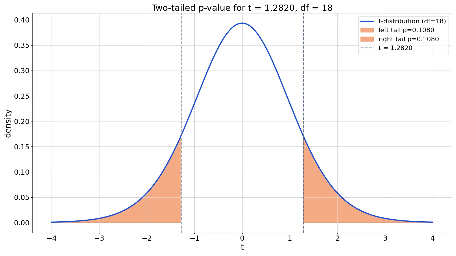
If you have a t statistic and want a p-value, you need two more things: the degrees of freedom and a decision about one-tailed or two-tailed. The conversion itself is just the area under the t-distribution curve beyond your t value. This article shows the formula, a full worked example, and how to do the t to p conversion in Excel, R and Python.

Quick Answer

The p-value is the tail area of the t-distribution beyond your t statistic, with df = n - 1 for a one-sample test [1].
Two-tailed p = $2 \times P(T > |t|)$. One-tailed p = $P(T > |t|)$ in the direction of your alternative hypothesis.
For the worked example here, t = 1.2820 with df = 18 gives a two-tailed p of 0.2161 and a one-tailed p of 0.1080.
In Python, 2 * stats.t.sf(abs(t), df) gives the two-tailed p. In Excel, =T.DIST.2T(ABS(t), df) does the same.
A large p-value means your data are consistent with the null hypothesis. It does not prove the null is true [2].

The Formula

The p-value for a t statistic is the probability that a t-distributed random variable with the same degrees of freedom is at least as extreme as the value you observed.

For a two-tailed test:

$$p = 2 \times P(T_{df} > |t|)$$

For a one-tailed test, when t falls on the side your alternative predicts (if it falls on the other side, the one-tailed p is 1 minus this value):

$$p = P(T_{df} > |t|)$$

Each symbol means the following.

$t$ is your computed t statistic, the standardized distance between your estimate and the null value.
$df$ is the degrees of freedom. For a one-sample t-test, $df = n - 1$. For a two-sample test, it depends on the variant you use.
$T_{df}$ is a random variable following the t-distribution with $df$ degrees of freedom.
$P(T_{df} > |t|)$ is the upper-tail area to the right of the absolute value of t.

The t-distribution is symmetric around zero, which is why the two-tailed p is exactly twice the one-tailed p when you use $|t|$ [1]. The shape depends on df. With small samples the tails are heavier, so the same t value gives a larger p than it would with a large sample.

How to Calculate It Step by Step

State the null and alternative hypotheses. The null is usually "no effect" or "the mean equals some value."
Decide whether the test is one-tailed or two-tailed. This must be decided before you look at the data.
Compute the t statistic. For a one-sample test, $t = (\bar{x} - \mu_0) / SE$, where $SE = s / \sqrt{n}$.
Find the degrees of freedom. For a one-sample t-test, $df = n - 1$.
Find the tail area. Use software, a table, or a calculator to get $P(T_{df} > |t|)$.
Double it for a two-tailed test. Leave it as is for a one-tailed test.
Compare the p-value to your alpha level, commonly 0.05, and report the result with the test details.

If you want to skip the manual steps, the P-Value Calculator takes a t statistic and degrees of freedom and returns both p-values.

Worked Example

The dataset is exam scores for 19 students, tested against a null hypothesis mean of 70.

student_id	score	student_id	score
1	72	11	70
2	65	12	66
3	80	13	79
4	68	14	73
5	74	15	67
6	71	16	76
7	69	17	64
8	77	18	78
9	63	19	72
10	75

The steps and their computed values:

Sample size: $n = 19$.
Degrees of freedom: $df = n - 1 = 18$.
Sample mean: $\bar{x} = 71.5263$.
Sample standard deviation: $s = 5.1894$.
Standard error: $SE = s / \sqrt{n} = 1.1905$.
t statistic: $t = (71.5263 - 70) / 1.1905 = 1.2820$.
Two-tailed p: $2 \times 0.1080 = 0.2161$.
One-tailed p: $0.1080$.
Critical t for a two-tailed test at alpha = 0.05: 2.1009.

Here is the same calculation in Python.

from scipy import stats
t = 1.2820
df = 18
p_two = 2 * stats.t.sf(abs(t), df)
p_one = stats.t.sf(abs(t), df)

Output:

p_two = 0.2161, p_one = 0.1080

The observed mean of 71.5263 is about 1.28 standard errors above 70. That is a modest distance. The t-distribution with 18 degrees of freedom puts about 10.8 percent of its area above 1.2820, so the two-tailed p is about 21.6 percent.

How to Interpret the Result

A p-value of 0.2161 means that if the true mean were exactly 70, you would see a t statistic at least this far from zero about 22 percent of the time in repeated samples. That is not rare. You would fail to reject the null at the usual 0.05 level.

The one-tailed p of 0.1080 is half the two-tailed value. It is still above 0.05, so the conclusion does not change here. But halving a p-value can flip a decision when the two-tailed p sits between 0.05 and 0.10, which is exactly why the choice must be made in advance.

The critical t value of 2.1009 gives you a second way to see the same result. Your t of 1.2820 is smaller than 2.1009, so it falls inside the non-rejection region. The p-value and the critical value approach always agree for the same test and alpha.

A p-value is not the probability that the null hypothesis is true, and it is not the size of the effect [2]. It measures compatibility between your data and a specified null model. Report the mean difference, the confidence interval and the sample size alongside it.

Doing It in Software (Excel, R or Python)

Excel has two functions that matter here.

=T.DIST.2T(ABS(t), df) returns the two-tailed p-value. It requires a non-negative t.
=T.DIST.RT(t, df) returns the right-tail area, which is the one-tailed p-value for an upper-tail test.

For the example, =T.DIST.2T(1.2820, 18) returns 0.2161 and =T.DIST.RT(1.2820, 18) returns 0.1080.

In R, pt() gives the cumulative distribution function, so you want the complement.

t <- 1.2820
df <- 18
p_two <- 2 * pt(abs(t), df, lower.tail = FALSE)
p_one <- pt(abs(t), df, lower.tail = FALSE)

In Python, stats.t.sf() is the survival function, which is the upper-tail area directly.

from scipy import stats
t = 1.2820
df = 18
p_two = 2 * stats.t.sf(abs(t), df)
p_one = stats.t.sf(abs(t), df)

If you are running the whole test instead of converting a single t value, stats.ttest_1samp in Python and t.test in R return the t statistic and p-value together. For a menu-driven route, see how to perform and interpret a t-test in SPSS.

Common Mistakes

Using the wrong degrees of freedom. For a one-sample test, df = n - 1. For a Welch two-sample test, df is not simply n1 + n2 - 2. Check which variant your software used.
Doubling a one-tailed p by mistake. If your software already returned a one-tailed p and you double it, you report a value twice as large as it should be. Know what the function returns.
Choosing the tail after seeing the data. Switching from two-tailed to one-tailed because the result was close to significant inflates your false positive rate. Fix the test before analysis.
Passing a negative t to T.DIST.2T. Excel returns an error for negative input. Wrap it in ABS().
Confusing the p-value with the probability the null is true. A p-value of 0.2161 does not mean there is a 21.6 percent chance the null holds [2].
Reporting a p-value without the test details. A p-value alone is uninterpretable without the test type, df, sample size and effect size.

Limitations

The t to p conversion assumes the test statistic really follows a t-distribution under the null. That holds for normal data or reasonably large samples by the central limit theorem. With small samples from heavily skewed data, the p-value can be misleading. The conversion also assumes your observations are independent. Clustered or repeated-measures data need a different model.

A p-value answers one narrow question about compatibility with a null model. It says nothing about practical importance, and a tiny p-value from a huge sample can accompany a trivial effect [2]. The conversion also cannot rescue a poorly designed study. If the sampling was biased or the hypothesis was chosen after looking at the data, an accurate p-value is still the wrong number to report.

Frequently Asked Questions

What is the difference between a one-tailed and two-tailed p-value?

A two-tailed p-value counts extreme values in both directions, so it is twice the one-tailed value when you use the absolute t. A one-tailed p-value counts only one direction, matching an alternative hypothesis that specifies a sign. Use two-tailed unless you have a strong directional prediction made before collecting data.

How do I convert t to p by hand?

You need a t-table or a calculator. Find the row for your degrees of freedom, locate where your t value falls between the critical values, and read off the tail probability. Exact values require software because tables only give a few columns. The t statistic formula article covers how to get the t value itself.

Can a t statistic be negative?

Yes. A negative t just means your sample estimate fell below the null value. For a two-tailed p-value, take the absolute value first. For a one-tailed test, the sign tells you which tail to use.

Why does my p-value change when df changes?

The t-distribution has heavier tails when df is small. The same t value therefore sits further out in a small-sample distribution, giving a larger p. As df grows, the t-distribution approaches the normal distribution. The Student's t-distribution guide explains how the shape depends on df.

Is a p-value of 0.05 the cutoff for significance?

It is a convention, not a law. Many fields use 0.05 as the threshold, but the right cutoff depends on the cost of errors and the study design. A p-value just above or below 0.05 is not meaningfully different from the other side of the line [2].

References

- Krzywinski M, Altman N (2013). Significance, P values and t-tests. Nature Methods
- Altman N, Krzywinski M (2017). Interpreting P values. Nature Methods
Further Reading
- NIST/SEMATECH e-Handbook of Statistical Methods
- Wasserstein RL, Lazar NA (2016). The ASA Statement on p -Values: Context, Process, and Purpose. The American Statistician
- OpenStax. Introductory Statistics 2e
- Krzywinski M, Altman N (2013). Importance of being uncertain. Nature Methods