What Is Skewness? Definition, Formula and Examples
By Dr. Zubair Khalid, DVM, MS, PhD ·
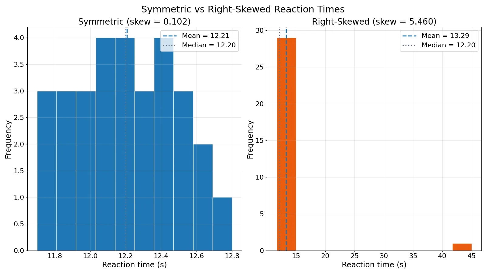
Skewness measures how lopsided a distribution is. A symmetric dataset has a skewness near zero, a long right tail gives a positive value, and a long left tail gives a negative value. The skew definition is that simple, but the number is only useful if you know what it is comparing and what it ignores.
Quick Answer
- Skewness is a single number that describes the asymmetry of a distribution. Zero means symmetric, positive means the right tail is longer, negative means the left tail is longer [1].
- The most common version is the Fisher-Pearson coefficient, built from cubed deviations from the mean divided by the cube of the standard deviation [1].
- Software usually reports the adjusted version, which corrects for sample size. The adjustment factor is 1.49 at n = 5, 1.19 at n = 10 and 1.08 at n = 20, and it approaches 1 as n grows [1].
- Skewness is sensitive to extreme values. One large outlier can move it a long way, as the worked example below shows.
- The sign tells you the direction of the tail, not where most of the data sits. In a right-skewed set, most values can still be below the mean.
What Skewness Means
In everyday language, the skew meaning is a tilt or a lean away from balance. In statistics it is the same idea applied to a frequency distribution: one side of the curve stretches out further than the other.
The precise statistical definition is that skewness is the third standardized moment of a distribution. A symmetric distribution is one in which the two halves of the histogram appear as mirror images of each other [2]. A skewed distribution is non-symmetric, and it is common for one tail to be considerably longer or more drawn out than the other [2].
Direction is named after the tail, not the bulk of the data. A skewed right distribution has its tail on the right side, and a skewed left distribution has its tail on the left side [2]. That naming convention trips up a lot of people, so it is worth repeating: you look at the thin, stretched-out end, not the tall, crowded end.
How It Works
The Fisher-Pearson coefficient of skewness is the standard formula [1]:
$$g_1 = \frac{\frac{1}{N}\sum_{i=1}^{N}(Y_i - \bar{Y})^3}{s^3}$$
Each symbol does a specific job:
- $N$ is the number of observations.
- $Y_i$ is the $i$-th data value.
- $\bar{Y}$ is the sample mean.
- $(Y_i - \bar{Y})$ is a deviation from the mean. Values above the mean are positive, values below are negative.
- The exponent 3 is what creates the asymmetry signal. Cubing keeps the sign of each deviation and amplifies large ones far more than small ones.
- $s$ is the standard deviation computed with $N$ in the denominator (not $N - 1$), and $s^3$ rescales the result so it does not depend on the units of measurement.
Because the deviations are cubed, a value far from the mean contributes a huge amount to the numerator. A value twice as far from the mean contributes eight times as much. That is why skewness reacts so strongly to outliers.
Many software programs compute the adjusted Fisher-Pearson coefficient instead, which multiplies the result by a factor that depends on sample size [1]. The adjustment approaches 1 as $N$ gets large [1]. For reference, the adjustment factor is 1.49 for $N = 5$, 1.19 for $N = 10$ and 1.08 for $N = 20$ [1]. SciPy's skew function computes the Fisher-Pearson coefficient and corrects for bias when bias is set to False [3].
Worked Example
The dataset is 30 lab reaction times in seconds. The first 29 values sit tightly between 11.7 and 12.8. The 30th value is 45.0, a single slow trial.
| Trial | Symmetric time (s) | Skewed time (s) |
|---|---|---|
| 1 | 12.1 | 12.1 |
| 2 | 12.4 | 12.4 |
| 3 | 11.8 | 11.8 |
| 4 | 12.6 | 12.6 |
| 5 | 12.2 | 12.2 |
| 6 | 11.9 | 11.9 |
| 7 | 12.5 | 12.5 |
| 8 | 12.0 | 12.0 |
| 9 | 12.3 | 12.3 |
| 10 | 12.1 | 12.1 |
| 11 | 11.7 | 11.7 |
| 12 | 12.8 | 12.8 |
| 13 | 12.2 | 12.2 |
| 14 | 12.4 | 12.4 |
| 15 | 11.9 | 11.9 |
| 16 | 12.3 | 12.3 |
| 17 | 12.1 | 12.1 |
| 18 | 12.5 | 12.5 |
| 19 | 12.0 | 12.0 |
| 20 | 12.2 | 12.2 |
| 21 | 12.6 | 12.6 |
| 22 | 11.8 | 11.8 |
| 23 | 12.4 | 12.4 |
| 24 | 12.1 | 12.1 |
| 25 | 12.3 | 12.3 |
| 26 | 12.0 | 12.0 |
| 27 | 12.5 | 12.5 |
| 28 | 12.2 | 12.2 |
| 29 | 11.9 | 11.9 |
| 30 | 12.4 | 45.0 |
Both columns have $n = 30$. The only difference is the last value.
For the symmetric column, the mean is 12.2067, the median is 12.2000, the sample standard deviation is 0.2716, and the skewness is 0.1019. The mean and median nearly coincide and the skewness is close to zero, which is what you expect from symmetric data [1].
For the skewed column, the mean rises to 13.2933 while the median stays at 12.2000. The standard deviation jumps to 5.9945. The sum of cubed deviations from the mean is 31830.4156, and the adjusted Fisher-Pearson skewness is:
$$g_1 = \frac{30}{(30-1)(30-2)} \times \frac{31830.4156}{5.9945^3} = 5.4595$$
That is a large positive value, and it matches what SciPy returns with bias=False.
from scipy import stats
import statistics

symmetric = [12.1, 12.4, 11.8, 12.6, 12.2, 11.9, 12.5, 12.0, 12.3, 12.1,
             11.7, 12.8, 12.2, 12.4, 11.9, 12.3, 12.1, 12.5, 12.0, 12.2,
             12.6, 11.8, 12.4, 12.1, 12.3, 12.0, 12.5, 12.2, 11.9, 12.4]
skewed = symmetric[:-1] + [45.0]

print('symmetric skew:', round(stats.skew(symmetric, bias=False), 4))
print('skewed skew:   ', round(stats.skew(skewed, bias=False), 4))
print('skewed mean:   ', round(statistics.mean(skewed), 4))
print('skewed median: ', round(statistics.median(skewed), 4))
symmetric skew: 0.1019
skewed skew: 5.4595
skewed mean: 13.2933
skewed median: 12.2000One value out of thirty moved the skewness from 0.1019 to 5.4595. The mean moved by more than a second while the median did not move at all.
How to Interpret It
Read the sign first, then the size.
- Near zero: the data are roughly symmetric. For normally distributed data, the skewness should be about zero [3].
- Positive: the right tail is longer. For unimodal continuous distributions, a skewness greater than zero means there is more weight in the right tail [3].
- Negative: the left tail is longer. Negative values indicate data that are skewed left, meaning the left tail is long relative to the right tail [1].
Size is harder to judge because there is no universal cutoff. The National Institute of Standards and Technology reports a dataset with a skewness of 1.08 and a kurtosis of 4.46 and describes it as indicating moderate skewness and kurtosis [1]. Values in the single digits can already signal a strongly lopsided shape.
A practical habit is to compare the mean and the median. When the mean sits well above the median, the distribution is usually right-skewed. When the mean sits well below the median, it is usually left-skewed. In the worked example the mean is 13.2933 and the median is 12.2000, a gap of more than a second that points straight at the right tail.
If you want to see the same idea drawn as a box plot, the article on reading a left-skewed box plot walks through the visual cues.
When to Use It (and when not to)
Use skewness when you are describing the shape of a distribution before choosing a statistical method. Many classical statistical tests and intervals depend on normality assumptions, and significant skewness is one of the signals that those assumptions may not hold [1]. It is also useful when you are deciding whether the mean or the median is the better summary of a typical value, since skewed distributions make that choice genuinely ambiguous [2].
Skip it, or treat it with suspicion, when your sample is very small. The adjustment factor is 1.49 at $N = 5$ and 1.19 at $N = 10$, which tells you the raw statistic is badly biased in small samples [1]. Skip it when you only need a rough sense of shape, since a histogram or a box plot communicates the same thing faster. And skip it when a single extreme value is driving the result and you have not yet decided whether that value is real data or an error.
Skewness vs Standard Deviation
These two are often confused because both describe a distribution's shape, but they answer different questions.
| Property | Skewness | Standard deviation |
|---|---|---|
| What it measures | Asymmetry, the balance of the two tails | Spread, the typical distance from the mean |
| Sign | Can be negative, zero or positive | Always zero or positive |
| Symmetric data | Near zero | Any value |
| Effect of one outlier | Can change dramatically | Increases, but less sharply |
| Units | None, it is standardized | Same units as the data |
A dataset can be perfectly symmetric and still have a large standard deviation. A dataset can be tightly clustered and still be strongly skewed. In the worked example, the symmetric column has a standard deviation of 0.2716 and the skewed column has 5.9945, so both numbers moved, but only the skewness tells you the movement was one-sided.
Common Mistakes
- Reading the sign as the side with more data. The sign follows the tail, not the peak. Fix: sketch the histogram and mark which end is stretched out.
- Assuming a positive skew means the mean is above every value. It usually means the mean is pulled above the median, although even that rule has exceptions. Fix: report the mean and median together.
- Comparing skewness across datasets with different sample sizes without checking the adjustment. The raw and adjusted versions differ most in small samples [1]. Fix: state which version your software reports.
- Treating any nonzero value as proof of non-normality. Sampling noise produces small nonzero values all the time. Fix: use a formal test such as
skewtestto judge whether a value is close enough to zero [3]. - Dropping an outlier just to make the skewness look better. The outlier may be the most informative observation in the set. Fix: report the skewness with and without it.
- Using skewness on data with two distinct peaks. A bimodal distribution can have a skewness near zero while being nothing like a normal curve. Fix: look at the histogram first.
Limitations
Skewness compresses the entire shape of a distribution into one number, and that number can hide a lot. A bimodal dataset can produce a skewness near zero even though it looks nothing like a symmetric bell curve. The statistic also says nothing about where the tails come from, so it cannot tell you whether a long right tail reflects genuine variation or a data entry error.
The statistic is also unstable in small samples and highly sensitive to extreme values. Just as the mean and standard deviation can be distorted by extreme values in the tails, so too can the skewness and kurtosis [1]. If your dataset has heavy tails, the skewness value itself may be dominated by a handful of points, which makes it a poor basis for decisions on its own. Pair it with a histogram, the mean, the median and the standard deviation before you draw conclusions.
Frequently Asked Questions
What is a simple skew definition?
Skewness is a measure of how asymmetric a distribution is. A value near zero means the two halves mirror each other, a positive value means the right tail is longer, and a negative value means the left tail is longer [1]. It is a single number that summarizes the shape of a dataset.
What does a negative skew mean?
A negative skew means the left tail is long relative to the right tail [1]. The bulk of the data sits toward the high end of the range, with a few unusually small values stretching the distribution to the left. The mean is typically pulled below the median.
Is skewness of 1 high?
There is no fixed threshold, but a value of 1 is generally treated as meaningful. The National Institute of Standards and Technology describes a skewness of 1.08 as indicating moderate skewness [1]. For a formal judgment, use a test such as skewtest to check whether the value is statistically distinguishable from zero [3].
How do I tell left skew from right skew?
Look at the longer tail. A skewed right distribution has its tail on the right side, and a skewed left distribution has its tail on the left side [2]. If you only have summary statistics, compare the mean and the median: mean above median suggests right skew, mean below median suggests left skew. The comparison between skew to the left and skewed right covers the visual checks in more detail.
Does skewness depend on the units of measurement?
No. The cubed deviations in the numerator are divided by the cube of the standard deviation, so the units cancel out. That makes skewness a unitless number you can compare across datasets measured in seconds, dollars or millimeters. The same is not true of the mean or the standard deviation, which keep the original units.
References
- 1.3.5.11. Measures of Skewness and Kurtosis
- 1.3.3.14.6. Histogram Interpretation: Skewed (Non-Normal) Right
- skew, SciPy v1.18.0 Manual
Further Reading
- NIST/SEMATECH e-Handbook of Statistical Methods
- OpenStax. Introductory Statistics 2e
- Krzywinski M, Altman N (2013). Importance of being uncertain. Nature Methods