What Is Discrete Data? Definition and Examples

By Dr. Zubair Khalid, DVM, MS, PhD · 2026-10-03

Quick Answer

Discrete data comes from counting. Each value is separate and countable, such as 3 customers, 12 defects or 0 goals.
Continuous data comes from measuring. It can take any value in a range, such as 4.2 minutes or 71.35 kilograms.
The test is simple: can the value be split into smaller meaningful parts? If yes, it is continuous. If no, it is discrete.
Discrete data is summarized with counts, frequencies and proportions. Continuous data is summarized with means, standard deviations and quartiles.
Discrete data is often modeled with contingency tables and log-linear models, while continuous responses are usually handled with classical linear models and ANOVA [1].

If you are asking "what is discrete data," the shortest honest answer is this: it is data you get by counting whole, separate items. You can have 4 support tickets or 5 support tickets, but never 4.6 support tickets. That single property drives almost every decision that follows, from which chart you draw to which statistical test you run.

What Discrete Data Means

In plain terms, discrete data is data whose possible values are distinct and countable. There is a gap between one value and the next, and nothing meaningful lives in that gap. The number of people in a room, the number of goals in a match and the number of errors in a log file are all discrete.

The precise statistical definition is narrower and more useful. A variable is discrete if its set of possible values is finite or countably infinite. Countably infinite means you could in principle list every value in order, even if the list never ends. The number of coin flips until the first head is discrete, because the possible values are 1, 2, 3 and so on, with no values in between.

Discrete data usually arises from counting, but it can also arise from labeling. A survey answer of "favor" or "oppose" is discrete, and so is a yield result of "good" or "bad" [1]. These are not numbers at all, yet they are still discrete because the outcomes are separate categories with no intermediate state.

This is why discrete data is a category of its own in statistics. When the response is discrete, the standard tools for continuous responses stop being appropriate [1]. You need methods built for counts and categories instead.

How It Works

The mechanism behind discrete data is the probability distribution that generates it. For counts, the most common choice is the Poisson distribution, which gives the probability of observing exactly $k$ events:

$$P(X = k) = \frac{\lambda^k e^{-\lambda}}{k!}$$

Each symbol means the following.

$X$ is the discrete random variable, such as the number of customers in a day.
$k$ is a specific non-negative integer you are asking about, such as 3.
$\lambda$ (lambda) is the mean number of events per unit of time or space.
$e$ is Euler's number, roughly 2.71828.
$k!$ is the factorial of $k$, the product of all integers from 1 to $k$.

The key feature is that $k$ only takes whole-number values. There is no term for $k = 3.5$, because half a customer is not an outcome the process can produce.

For discrete categories, the equivalent tool is the contingency table. A contingency table cross-tabulates two discrete variables, such as process A versus process B against pass versus fail, and a chi-square test checks whether the two classifying variables are independent [1]. If the test statistic is below the chi-square critical value at your chosen significance level, you fail to reject independence, which means the data show no significant association but do not prove independence. Otherwise you conclude the variables are associated [1].

When you have both discrete and continuous explanatory variables, the standard approach is a log-linear model [1]. That is the practical bridge between the two data types.

Worked Example

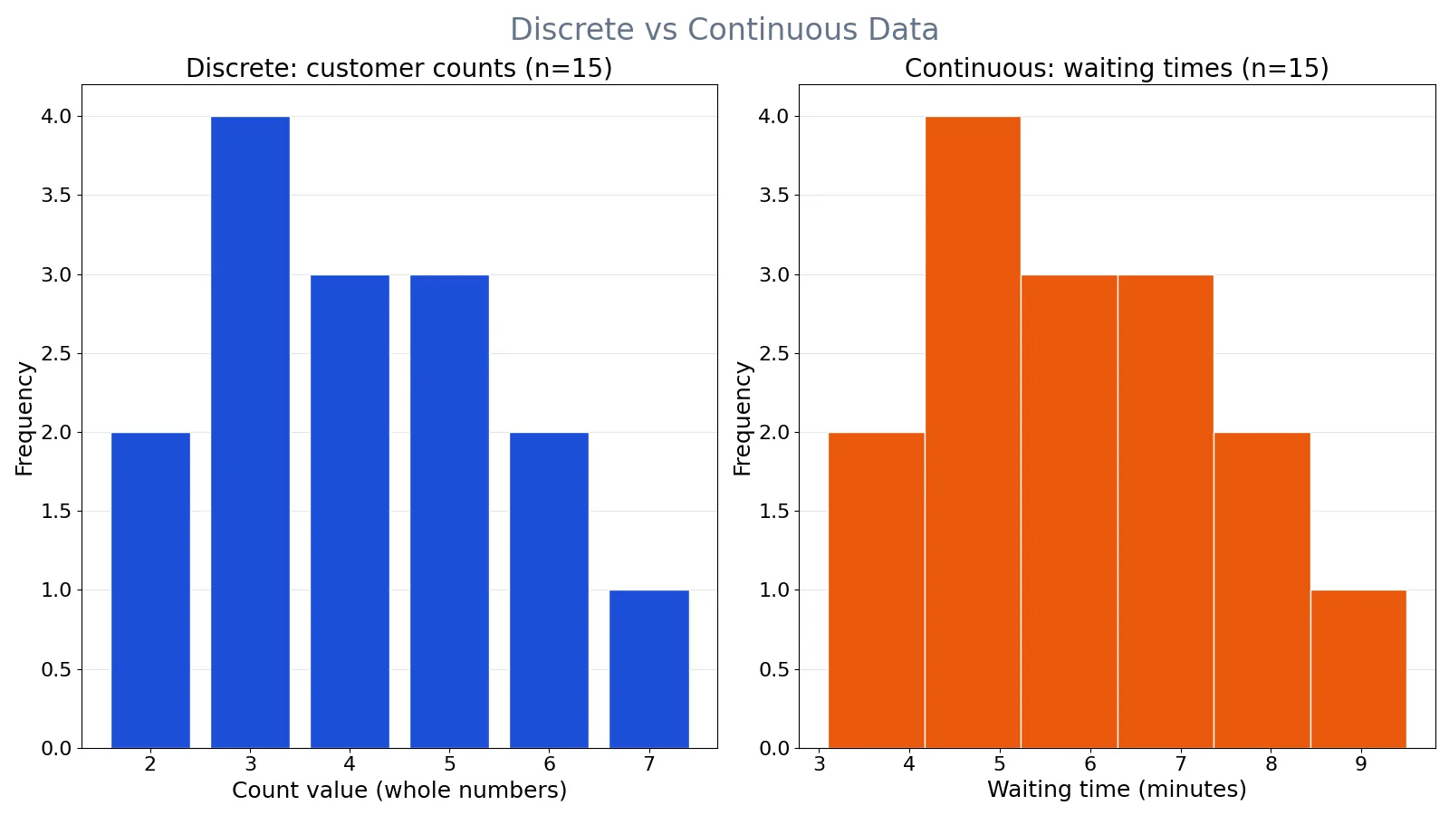
The dataset below records daily customer counts (discrete) and average waiting times in minutes (continuous) over 15 days at a small service counter.

day	customer_count	wait_minutes
1	3	4.2
2	5	6.8
3	2	3.1
4	7	9.5
5	4	5.4
6	3	7.2
7	5	4.9
8	3	6.1
9	6	8.3
10	4	5.7
11	2	3.8
12	5	7.9
13	3	4.5
14	4	6.6
15	6	5.2

Step 1: list the distinct values in the discrete column. The unique counts are 2, 3, 4, 5, 6 and 7. Only six values appear across 15 days, and every one is a whole number.

Step 2: count how often each value occurs. The frequency table is 2 appears twice, 3 appears four times, 4 appears three times, 5 appears three times, 6 appears twice and 7 appears once. Those frequencies sum to 15, which matches the total number of observations.

Step 3: summarize the discrete column. The mean customer count is 4.1333, the median is 4.0000 and the mode is 3. The sample variance is 2.2667 and the sample standard deviation is 1.5055.

Step 4: summarize the continuous column for contrast. The mean waiting time is 5.9467 minutes with a standard deviation of 1.7848. The first quartile is 4.7000 and the third quartile is 7.0000, giving an interquartile range of 2.3000.

Step 5: reproduce it in code.

import statistics
counts = [3, 5, 2, 7, 4, 3, 5, 3, 6, 4, 2, 5, 3, 4, 6]
waits = [4.2, 6.8, 3.1, 9.5, 5.4, 7.2, 4.9, 6.1, 8.3, 5.7, 3.8, 7.9, 4.5, 6.6, 5.2]
print(statistics.mean(counts))   # 4.1333
print(statistics.stdev(counts))  # 1.5055
print(statistics.mean(waits))    # 5.9467
print(statistics.stdev(waits))   # 1.7848

Output:

4.133333333333334
1.505545305418162
5.946666666666667
1.7848035772946584

The same numbers come out of a spreadsheet. In Excel, =ROUND(AVERAGE(A2:A16),2) returns 4.13, =ROUND(STDEV.S(A2:A16),4) returns 1.5055, =MEDIAN(A2:A16) returns 4.0, =MODE(A2:A16) returns 3 and =COUNT(A2:A16) returns 15.

In SQL, a grouped count gives the same frequency table: [(2, 2), (3, 4), (4, 3), (5, 3), (6, 2), (7, 1)]. A summary row returns (15, 4.133333333333334, 2, 7), meaning 15 rows, a mean of about 4.13, a minimum of 2 and a maximum of 7.

Notice what the two columns do differently. The customer counts land on six exact values, and the mode is meaningful because 3 is genuinely the most common day. The waiting times spread across a range with no repeats at all, so a mode would be useless and the quartiles carry the information instead.

How to Interpret It

Read a discrete summary through frequencies first. The frequency table tells you the shape of the distribution, and the mode tells you the most common outcome. A mean of 4.13 customers is useful, but the fact that 3 customers occurred on 4 of 15 days is often the more actionable number.

Read a continuous summary through spread. The mean waiting time of 5.95 minutes means little on its own. The interquartile range of 2.30 minutes tells you that the middle half of days fell between 4.70 and 7.00 minutes, which is what a customer actually experiences.

The distinction also changes what a "difference" means. With discrete counts, a difference of 1 is a real, indivisible step. With continuous measurements, a difference of 1 minute is a slice of a range, and the same underlying process could easily produce 1.02 or 0.98.

When to Use It (and when not to)

Treat your data as discrete when the values are counts or categories and the gaps between them are real. This applies to defect counts, ticket volumes, survey responses, pass or fail outcomes and any variable where fractional values are impossible.

Treat your data as continuous when the values come from a measurement instrument and any value in a range is possible. Time, weight, temperature, distance and percentage scores usually fall here.

The choice matters because it determines your method. Classical linear models and ANOVA assume a continuous response, and they are not appropriate when the response is discrete [1]. For discrete responses you move to contingency table analysis when the explanatory variables are also discrete, or to log-linear models when you have a mix of discrete and continuous predictors [1].

One practical warning. A variable can be recorded as discrete and still behave continuously. If you group waiting times into bins of "slow," "fast" and "faster," you have created discrete data from a continuous source [1]. That is a legitimate modeling choice, but it throws away information, so make it deliberately.

Discrete Data vs Continuous Data

Property	Discrete data	Continuous data
Origin	Counting or labeling	Measuring
Possible values	Separate, countable values	Any value in a range
Example from the dataset	Customer count: 2, 3, 4, 5, 6, 7	Waiting time: 4.2, 6.8, 3.1 minutes
Mean	4.1333	5.9467
Standard deviation	1.5055	1.7848
Mode	Meaningful, equals 3	Usually meaningless
Quartiles	Often not useful	Q1 = 4.7000, Q3 = 7.0000
Typical chart	Bar chart	Histogram
Typical model	Contingency table, log-linear model	Linear model, ANOVA

The mode row is the clearest tell. In the discrete column, 3 is a genuine peak. In the continuous column, no waiting time repeats, so a mode would be an artifact of rounding.

Common Mistakes

Treating a count as continuous and running a t-test or ANOVA on it. Counts violate the continuous-response assumption, so use contingency table analysis or a log-linear model instead [1].
Averaging a discrete variable and reporting a fractional result as if it were observable. A mean of 4.13 customers is a valid summary, but no day had 4.13 customers.
Reporting a mode for continuous data. If every value is unique, the mode is noise. Use the median and quartiles instead.
Assuming whole numbers always mean discrete. A weight recorded as 70 kg is continuous data that happens to be rounded. The underlying variable is still continuous.
Binning a continuous variable and then analyzing it as discrete without saying so. Binning is a modeling decision, and it discards detail.
Confusing discrete with categorical. Ordinal and nominal data are discrete, but not all discrete data is categorical. Counts are discrete and numeric.

Limitations

Discrete data summaries lose information in ways continuous summaries do not. Once you collapse counts into a mean, you hide the shape of the distribution, and for counts the shape often matters more than the center. A mean of 4 customers could come from a steady 4 every day or from alternating 2s and 6s, and those are very different businesses.

The methods built for discrete responses also carry their own assumptions. Chi-square results in contingency tables start to break down under certain conditions, and the estimation and testing results hold regardless of whether the underlying model is Poisson, multinomial or product-multinomial only within those limits [1]. As you add factors to a contingency table, interpretation becomes harder even though the arithmetic still works [1].

Frequently Asked Questions

Is discrete data always a whole number?

No. Discrete data is countable, which usually means whole numbers, but the defining property is that the values are separate. A rating scale of 1.0, 1.5, 2.0 and so on is discrete if those are the only permitted values, because nothing exists between them.

What is discrete data in simple terms?

It is data you get by counting separate things. You can count 3, 4 or 5 support tickets, but you cannot have 4.6 tickets. Each possible value is distinct, and there is nothing meaningful in the gap between one value and the next.

Can discrete data be averaged?

Yes, but read the result carefully. The mean customer count of 4.1333 is a legitimate summary of 15 days, yet it describes no single day. Pair the mean with the frequency table so the reader sees the actual outcomes.

How do I know if my data is discrete or continuous?

Ask whether a value between two observations is possible and meaningful. If 4.5 customers is impossible, the data is discrete. If 4.5 minutes is a real waiting time someone could experience, the data is continuous.

What is the difference between discrete data and categorical data?

Categorical data is a subset of discrete data. Categories like "favor" and "oppose" are discrete because the outcomes are separate [1]. Counts like 3 customers are also discrete, but they are numeric, so you can add and average them in ways you cannot with labels.

References

3.2.4. Discrete Models