Probability of A Given B: Conditional Probability Formula and Examples

By Dr. Zubair Khalid, DVM, MS, PhD · 2026-10-03

The probability of A given B answers a narrower question than the plain probability of A. It asks how likely A is once you already know that B happened, so the sample space shrinks from everything that could occur to only the outcomes inside B. The formula is $P(A \mid B) = \dfrac{P(A \cap B)}{P(B)}$, and it is valid whenever $P(B) > 0$ [1].

Quick Answer

The probability of A given B is written $P(A \mid B)$ and read "the probability of A given B" [2].
Formula: $P(A \mid B) = \dfrac{P(A \cap B)}{P(B)}$, the probability that both events occur divided by the probability of the condition [1].
The condition B becomes the new sample space. You count only outcomes inside B [2].
If A and B are independent, knowing B changes nothing, so $P(A \mid B) = P(A)$ [3].
Rearranged, the same rule gives the multiplication rule $P(A \cap B) = P(A) \cdot P(B \mid A)$ [4].

The Formula

$$P(A \mid B) = \frac{P(A \cap B)}{P(B)}$$

Each symbol means something specific:

Symbol	Meaning
$A$	The event you want the probability of
$B$	The event you already know happened, called the condition
$A \cap B$	The intersection, meaning both A and B occur together
$P(A \cap B)$	The joint probability of A and B
$P(B)$	The unconditional probability of B
$P(A \mid B)$	The conditional probability of A given B

The denominator is the key. Dividing by $P(B)$ rescales the joint probability so that the total probability inside B becomes 1. That is why the condition is described as a restricted or reduced sample space [1].

The formula only works when $P(B) > 0$. If B cannot happen, conditioning on it is undefined [1].

How to Calculate It Step by Step

Define A and B in words before touching any numbers. Ambiguity here causes most errors.
Find $P(B)$, the probability of the condition. This is the denominator.
Find $P(A \cap B)$, the probability that both events happen together. This is the numerator.
Divide the joint probability by the probability of B.
Check that the answer lies between 0 and 1. A result outside that range means an arithmetic or setup error.
Sanity-check the direction. $P(A \mid B)$ and $P(B \mid A)$ are usually different numbers.

If you have raw counts instead of probabilities, you can skip the probability step entirely. Count the cases where both A and B occur, then divide by the count of cases where B occurs. The probabilities cancel out, so the ratio is identical.

Worked Example

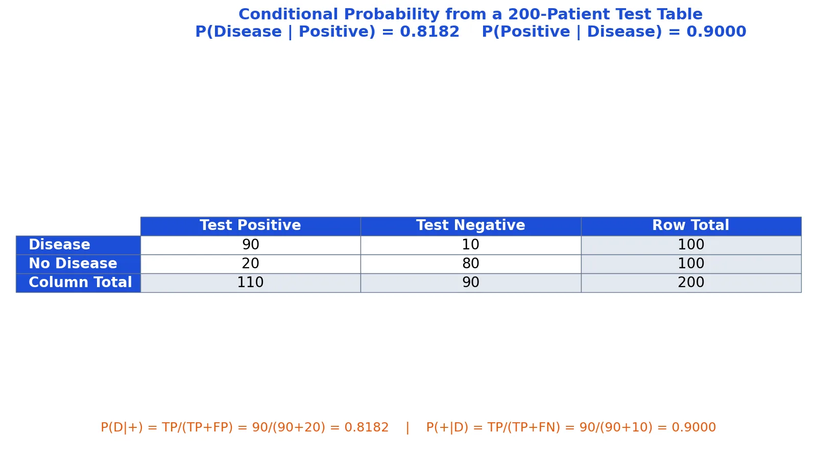
A clinic tests 200 patients for a disease. Each patient has a test result and a confirmed disease status, giving four groups.

Test Result	Disease Status	Count
Positive	Disease	90
Positive	No Disease	20
Negative	Disease	10
Negative	No Disease	80

The four counts are 90 true positives, 20 false positives, 10 false negatives, and 80 true negatives, for 200 patients total.

Let A be "has the disease" and B be "tests positive." We want the probability of A given B, which is the chance a patient actually has the disease given a positive test.

Step 1. Total patients. $N = 200$.

Step 2. Probability of disease given a positive test. Restrict to the 110 patients who tested positive. Of those, 90 have the disease.

$$P(\text{Disease} \mid \text{Positive}) = \frac{90}{90 + 20} = \frac{90}{110} = 0.8182$$

Step 3. Probability of a positive test given disease. Now restrict to the 100 patients who have the disease. Of those, 90 tested positive.

$$P(\text{Positive} \mid \text{Disease}) = \frac{90}{90 + 10} = \frac{90}{100} = 0.9000$$

Step 4. Unconditional probabilities. $P(\text{Disease}) = \dfrac{90 + 10}{200} = \dfrac{100}{200} = 0.5000$ and $P(\text{Positive}) = \dfrac{90 + 20}{200} = \dfrac{110}{200} = 0.5500$.

Step 5. Joint probability. $P(\text{Disease and Positive}) = \dfrac{90}{200} = 0.4500$.

Step 6. Apply the formula. $\dfrac{0.4500}{0.5500} = 0.8182$, matching Step 2.

Step 7. Bayes check. The same answer comes from the other direction: $\dfrac{P(\text{Positive} \mid \text{Disease}) \cdot P(\text{Disease})}{P(\text{Positive})} = \dfrac{0.9000 \times 0.5000}{0.5500} = 0.8182$.

Notice that $P(\text{Disease} \mid \text{Positive}) = 0.8182$ and $P(\text{Positive} \mid \text{Disease}) = 0.9000$ are different numbers. The test is more sensitive than the result is conclusive, because 20 healthy patients still tested positive.

How to Interpret the Result

A value of 0.8182 means that among patients who test positive, about 81.8% actually have the disease. It does not mean 81.8% of all patients are sick, and it does not mean the test is 81.8% accurate. Those are different quantities.

The condition defines the group you are talking about. Every conditional probability is a statement about a subgroup, so always name the subgroup when you report it. "82% of positive-test patients have the disease" is a clear claim. "82% have the disease" is a different and false claim about this dataset.

Conditional probability is also the foundation of Bayes' theorem, which flips the condition to go from $P(B \mid A)$ to $P(A \mid B)$ [3]. That reversal is exactly what Step 7 did.

Doing It in Software

With counts, the calculation is a single division. This Python snippet uses the four counts from the table.

TP, FP, FN, TN = 90, 20, 10, 80
p_disease_given_pos = TP / (TP + FP)
p_pos_given_disease = TP / (TP + FN)
print(f"P(Disease | Positive) = {p_disease_given_pos:.4f}")
print(f"P(Positive | Disease) = {p_pos_given_disease:.4f}")

Output:

P(Disease | Positive) = 0.8182
P(Positive | Disease) = 0.9000

In Excel, if the true positive count sits in cell A1 and the false positive count in A2, the formula =A1/(A1+A2) returns 0.8182. In R, the same division works on numeric vectors, and prop.test handles the interval estimation when you need a confidence interval around the proportion.

For a quick check on any conditional probability problem, the Probability Calculator lets you enter the joint and marginal probabilities and returns the conditional value directly.

Common Mistakes

Flipping the condition. $P(A \mid B)$ and $P(B \mid A)$ are different quantities. In the example they are 0.8182 and 0.9000. Fix: write the condition in words before substituting numbers.
Dividing by the wrong total. Using the full sample size instead of the count inside B gives 90/200 = 0.45, which is the joint probability, not the conditional one. Fix: the denominator is always the size of the condition group.
Assuming independence without checking. If A and B are independent, $P(A \mid B) = P(A)$ [3]. That is a special case, not a default. Fix: verify independence or use the full formula.
Confusing the joint with the conditional. $P(A \cap B)$ is "both happen." $P(A \mid B)$ is "A happens inside the world where B happened." Fix: check whether your denominator is 1 or $P(B)$.
Conditioning on a zero-probability event. If $P(B) = 0$, the formula is undefined [1]. Fix: confirm the condition can actually occur before computing.
Ignoring base rates. A high $P(\text{Positive} \mid \text{Disease})$ does not guarantee a high $P(\text{Disease} \mid \text{Positive})$ when the disease is rare. Fix: always bring in the unconditional probability of the condition.

Limitations

Conditional probability describes association inside a defined group. It does not establish causation, and it cannot correct for a biased sample. If the 200 patients were not representative of the population you care about, the 0.8182 figure applies only to a group like this one.

The formula also depends on knowing $P(B)$ accurately. When the condition is rare, small errors in that estimate swing the conditional probability a lot. And when events are not independent, you cannot multiply their plain probabilities to get the joint probability. You need the conditional form of the multiplication rule instead [4].

Frequently Asked Questions

What is the difference between P(A|B) and P(B|A)?

They condition on different events and usually give different answers. $P(A \mid B)$ restricts the sample space to B, while $P(B \mid A)$ restricts it to A. In the worked example, $P(\text{Disease} \mid \text{Positive}) = 0.8182$ but $P(\text{Positive} \mid \text{Disease}) = 0.9000$. Bayes' theorem is the tool that converts one into the other [3].

What does "probability of A given B" mean in plain words?

It means the chance that A happens, calculated only among the cases where B already happened. The condition removes every outcome outside B from consideration. If you roll a die and learn the result is even, the probability of a 6 becomes 1/3 instead of 1/6, because only three outcomes remain [2].

Can conditional probability be greater than the unconditional probability?

Yes. Conditioning can raise or lower a probability. If B is positively associated with A, then $P(A \mid B)$ exceeds $P(A)$. If the two are independent, they are equal [3]. The only hard rule is that the result stays between 0 and 1.

What happens if P(B) equals zero?

The conditional probability is undefined, because the formula divides by zero [1]. Conditioning on an impossible event has no meaning. In practice, check that the condition has a nonzero probability before you compute anything.

How is conditional probability used in real analysis?

It appears wherever you filter data by a known characteristic. Medical testing, credit scoring, spam filtering, and survey subgroup analysis all rely on it. The multiplication rule $P(A \cap B) = P(A) \cdot P(B \mid A)$ extends the idea to chains of dependent events, such as drawing cards without replacement [4]. Related distributions such as the binomial distribution build directly on repeated independent trials, and Bayes' theorem handles the reversal of the condition.