How to Create a Drop Down List in Excel (Step by Step)

By Dr. Zubair Khalid, DVM, MS, PhD · 2026-10-03

A drop-down list in Excel is built with Data Validation. You type the allowed values in a range, select the cells that should offer the list, and point Data Validation at that range. This guide shows how to create a drop down in Excel step by step, then covers the errors that break it.

Quick Answer

Put the allowed values in a column or row, for example Open, In Progress, Closed in F2:F4.
Select the cells that should show the list, for example C2:C7.
Go to Data > Data Validation > Data Validation.
On the Settings tab, set Allow to List and set Source to =$F$2:$F$4.
Keep In-cell dropdown checked and click OK. Each selected cell now shows an arrow with the three values.

Before You Start

A drop-down list is not a separate Excel feature. It is one setting inside Data Validation, which controls what a user is allowed to type into a cell. When you set Allow to List, Excel compares every entry against a source list and rejects anything that is not on it.

Two things make the setup easier. First, decide where the allowed values live. A small block on the same sheet works well, and a separate sheet works if you do not want users to see or edit the list. Second, decide which cells get the list. You can select a single cell, a column of cells, or a whole table column.

The source range can be typed directly into the Source box, or you can click into the box and then drag over the cells. Typing the range with dollar signs, like =$F$2:$F$4, locks the reference so it does not shift if you copy the validation to other cells.

If you are still getting comfortable with cell references, the mechanics are the same as any other formula. See how to make a formula in Excel for the basics of relative and absolute references.

Step by Step

Type the allowed values. Enter each permitted value in its own cell, one per row or one per column. In the example below, the three status values go in F2, F3, and F4. Leave no blank cells inside the range, because a blank in the middle of the source list creates a blank option in the drop-down.

Select the target cells. Highlight the cells that should offer the list. For a status column, select C2:C7. You can select non-adjacent cells by holding Ctrl while clicking, and the same validation applies to all of them.

Open Data Validation. Go to Data > Data Validation > Data Validation. The dialog opens on the Settings tab.

Set Allow to List. In the Allow box, choose List. A Source box appears below it.

Enter the source range. Type =$F$2:$F$4 in the Source box, or click the box and drag over F2:F4. The dollar signs keep the reference fixed.

Check In-cell dropdown. The In-cell dropdown box should be checked. If it is unchecked, the validation still works but no arrow appears, so users have to type a valid value blind.

Click OK. Select a target cell such as C2 and click the arrow. The three values appear.

Test a rejection. Type an invalid value into one of the cells, such as Pending. Excel blocks it and shows the error alert you configured. This confirms the rule is active.

For a broader look at the rules you can attach to cells, including input messages and custom formulas, see Data Validation in Excel: How to Add Dropdown Lists and Rules.

Worked Example

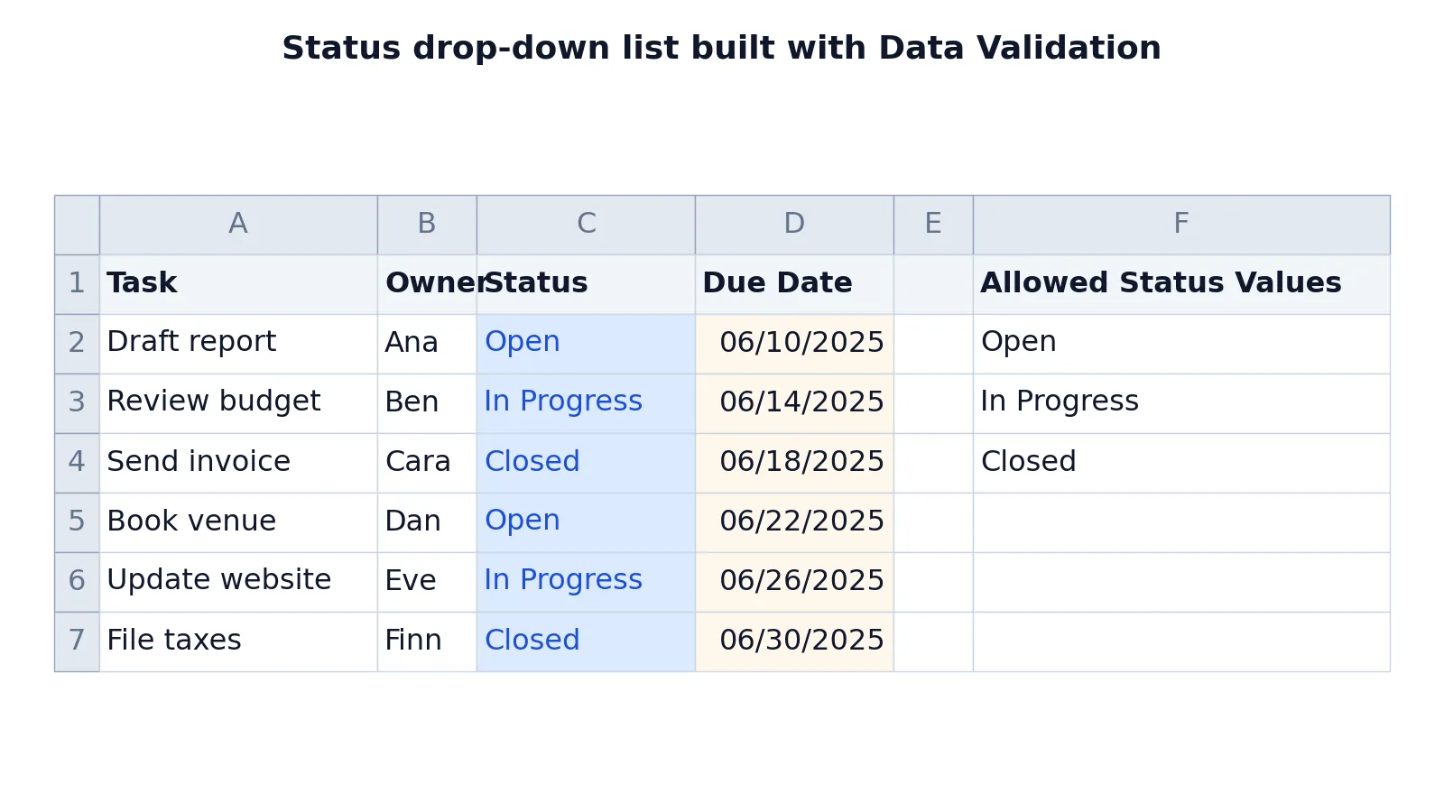
The sheet below tracks six tasks with an owner, a status, and a due date. The Status column is the one that gets the drop-down, sourced from the allowed values in F2:F4.

	A	B	C	D	F
1	Task	Owner	Status	Due Date	Allowed Status Values
2	Draft report	Ana	Open	`=DATE(2025,6,10)` -> displays 06/10/2025	Open
3	Review budget	Ben	In Progress	`=DATE(2025,6,14)` -> displays 06/14/2025	In Progress
4	Send invoice	Cara	Closed	`=DATE(2025,6,18)` -> displays 06/18/2025	Closed
5	Book venue	Dan	Open	`=DATE(2025,6,22)` -> displays 06/22/2025
6	Update website	Eve	In Progress	`=DATE(2025,6,26)` -> displays 06/26/2025
7	File taxes	Finn	Closed	`=DATE(2025,6,30)` -> displays 06/30/2025

The Due Date column uses the DATE function, which returns a real date serial number that Excel displays in your regional date format. The formula =DATE(2025,6,10) returns 06/10/2025, =DATE(2025,6,14) returns 06/14/2025, =DATE(2025,6,18) returns 06/18/2025, =DATE(2025,6,22) returns 06/22/2025, =DATE(2025,6,26) returns 06/26/2025, and =DATE(2025,6,30) returns 06/30/2025. Because these are true dates, you can sort and filter them chronologically instead of alphabetically.

The four steps that build the list are:

Type the three allowed status values in F2:F4 to use as the source list.
Select C2:C7, then open Data > Data Validation to restrict entries to the list in F2:F4.
In the Data Validation dialog, choose Allow: List and set Source to =$F$2:$F$4.
Click OK. Each Status cell now shows a drop-down arrow with Open, In Progress, and Closed.

The interface steps in full:

Select cells C2:C7 on the sheet.
Go to Data > Data Validation > Data Validation.
In the Settings tab, set Allow to List.
In the Source box, type =$F$2:$F$4.
Make sure In-cell dropdown is checked, then click OK.
Click a Status cell such as C2 to confirm the drop-down arrow appears.

Once the list is in place, the Status column is consistent. Every entry is one of three exact strings, so counting tasks by status with COUNTIF gives clean totals, and filtering the column returns tidy groups. The same idea applies when you filter in Excel, where a controlled vocabulary in one column makes the filter menu short and predictable.

Other Ways to Do It

Type the values directly into Source. Instead of pointing at a range, you can type the values separated by commas, for example Open,In Progress,Closed. This is fine for a short, fixed list. The downside is that the values are buried inside the validation rule, so nobody can see or edit them on the sheet.

Use a named range. Define a name for F2:F4, then set Source to =StatusList. The rule reads more clearly and survives row insertions better than a hard-coded range.

Use a table column as the source. If the allowed values live in an Excel table and Source points at that column's cells (directly or through a named range), the reference expands automatically when you add new values. This is the cleanest option when the list grows over time.

Copy the validation to other cells. Select a cell that already has the rule, copy it, then paste special with Validation selected onto the new cells. This avoids rebuilding the rule by hand.

Troubleshooting

The arrow does not appear. Check that In-cell dropdown is checked in the Data Validation dialog. If it is checked and the arrow is still missing, the cell may be formatted or protected in a way that hides it, or you may be looking at a cell outside the applied range.

Excel rejects the Source entry. The Source box expects either a range reference or a comma-separated list, not both. A reference must start with an equals sign, like =$F$2:$F$4. A plain list must not start with an equals sign.

The drop-down shows a blank option. There is a blank cell inside the source range. Shrink the range so it covers only the populated cells, or fill the blank.

The list does not update when you add a value. The source range is fixed, so a new value typed just below F4 falls outside it. Extend the range, or switch to a table column or named range that grows on its own.

Values typed earlier are now invalid. Data Validation applies to new entries. Existing values that are not on the list stay in the cell until you edit it. To find them, use Data > Data Validation > Circle Invalid Data.

The rule disappeared after a paste. Pasting ordinary cell contents over a validated cell replaces the validation. Use paste special with Validation selected when you want to carry the rule across.

Common Mistakes

Leaving a blank cell in the source range. This adds an empty option to the drop-down. Fix it by tightening the range to the populated cells only.
Using a relative reference in Source. =F2:F4 shifts when the rule is copied to other cells. Fix it with absolute references, =$F$2:$F$4.
Typing values with inconsistent spacing or case. Open and open are different strings to Excel, so counts and filters split. Fix it by standardizing the source list and picking from the drop-down instead of typing.
Pointing the source at the same cells you are validating. A circular reference like validating C2:C7 against C2:C7 breaks the rule. Fix it by keeping the source list in a separate range.
Forgetting that validation does not clean existing data. Old entries that are not on the list remain. Fix it by reviewing the column and correcting outliers manually.
Assuming validation is a security control. Anyone can paste over a validated cell or clear the rule. Treat it as a data-entry aid, not protection.

Limitations

Data Validation controls typing, not pasting. If a user copies a value from elsewhere and pastes it into a validated cell, Excel accepts it without checking the list. The same applies to values written by a macro or imported from another file. So a drop-down improves consistency at the point of entry, but it does not guarantee that a column is clean.

The source list is also a snapshot of the values you defined. If the business adds a new status, the drop-down keeps offering the old three until you update the range. And a drop-down cannot enforce relationships between columns, so it will not stop someone from marking a task Closed while the due date is still in the future. For rules like that you need a custom validation formula or a separate check column.

Frequently Asked Questions

How do I create a drop-down list in Excel from another sheet?

Put the allowed values on the second sheet, then in the Source box type the sheet name and range, for example =Sheet2!$A$2:$A$4. If the sheet name contains spaces, wrap it in single quotes, like ='Allowed Values'!$A$2:$A$4. The drop-down on the first sheet then reads from the second sheet.

Why is my drop-down arrow not showing in Excel?

The most common cause is that In-cell dropdown is unchecked in the Data Validation dialog. Open Data > Data Validation > Data Validation, go to the Settings tab, and check the box. Also confirm the cell you are looking at is inside the range you applied the rule to.

Can I make a drop-down that depends on another drop-down?

Yes. This is called a dependent or cascading drop-down. You build one list of categories and one list per category, then use a formula such as INDIRECT in the Source box so the second list changes based on the first selection. It takes more setup than a single list.

How do I edit or remove a drop-down list?

Select the cells, open Data > Data Validation > Data Validation, and change the Source range or the Allow setting. To remove the list entirely, click Clear All in the dialog and then OK. Clearing removes the rule but leaves the existing cell values in place.

Does a drop-down list stop people from typing other values?

It stops typing when the error alert is set to Stop, which is the default. You can relax this in the Error Alert tab by choosing Warning or Information, which lets an invalid entry through after a prompt. Pasting is never blocked by the list itself.

References

This article draws on the standard references listed under Further Reading.