Fitted Values in R: How to Extract and Interpret Them

By Dr. Zubair Khalid, DVM, MS, PhD · 2026-10-03

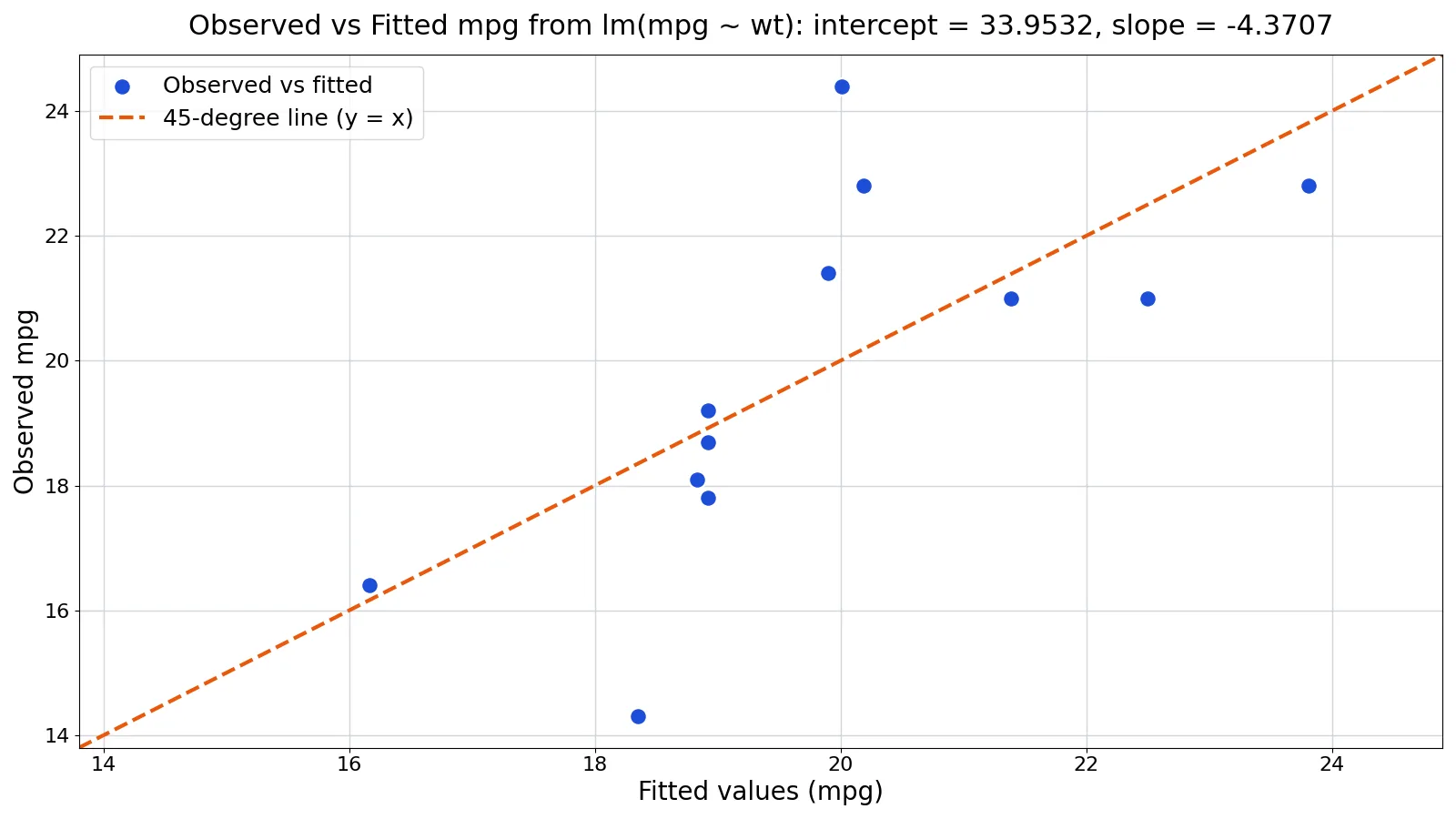
If you have fit a linear model in R, fitted() gives you the model's predicted response for every row that was used to build it. Each r fitted value is the height of the regression line at that observation's predictor value. This article shows the syntax, a worked example with real numbers, and the mistakes that trip people up.

Quick Answer

fitted(model) returns a numeric vector with one value per observation used in the fit [1].
fitted.values(model) is the same thing. fitted.values is the older name, and fitted is the generic function that most model classes implement [1][2].
A fitted value is computed as $\hat{y}_i = \hat{\beta}_0 + \hat{\beta}_1 x_i$ for a simple linear regression.
The residual is observed minus fitted, so residuals(model) equals mtcars$mpg - fitted(model) for complete cases.
Fitted values are in-sample predictions. They are not the same as predict(model, newdata = ...), which scores new rows.

Syntax

fitted() is a generic function, so the arguments depend on the method that runs for your model class. For lm objects the signature is simple [1][2].

Argument	Required?	Meaning
`object`	Yes	A fitted model object, such as the result of `lm()`, `glm()`, or `nls()` [1].
`...`	No	Extra arguments passed to the underlying method. Most `lm` calls need none.

The call returns a named numeric vector. The names come from the row names of the data used in the fit, which makes it easy to match a fitted value back to its source row.

How It Works

When you call lm(mpg ~ wt, data = mtcars), R builds a model matrix from the predictors and estimates coefficients by least squares. The fitted values are the product of that model matrix and the coefficient vector. In matrix form:

$$ \hat{y} = X\hat{\beta} $$

For a single predictor this collapses to the familiar line equation. The intercept is the predicted response when the predictor is zero, and the slope is the change in the predicted response per one-unit change in the predictor.

Two details matter in practice. First, fitted() returns values only for rows that survived any missing-value handling. If your data had NA in a variable, that row is dropped from the fit and the returned vector is shorter than your original data frame [3]. Second, the generic dispatches to a method, so fitted() works on many model types beyond lm, including generalized linear models and nonlinear least squares fits [1][2].

The values themselves are on the scale of the response variable. For lm that is the raw response. For a glm with a log link, the default fitted() returns values on the response scale, not the linear predictor scale.

Worked Example

The example uses a 12-row subset of mtcars with mpg and wt for each car.

car	mpg	wt
Mazda RX4	21.0	2.620
Mazda RX4 Wag	21.0	2.875
Datsun 710	22.8	2.320
Hornet 4 Drive	21.4	3.215
Hornet Sportabout	18.7	3.440
Valiant	18.1	3.460
Duster 360	14.3	3.570
Merc 240D	24.4	3.190
Merc 230	22.8	3.150
Merc 280	19.2	3.440
Merc 280C	17.8	3.440
Merc 450SE	16.4	4.070

Fit the model and extract the fitted values.

cars12 <- mtcars[1:12, ]   # the 12 cars in the table above
model <- lm(mpg ~ wt, data = cars12)
coef(model)
summary(model)$r.squared
round(fitted(model), 4)

Output:

Intercept: 33.9532
Slope: -4.3707
R^2: 0.4714
fitted(model): 22.5020, 21.3875, 23.8132, 19.9015, 18.9181, 18.8307, 18.3499, 20.0108, 20.1856, 18.9181, 18.9181, 16.1646

Walk through the first row. The formula is:

$$ \hat{\text{mpg}} = 33.9532 + (-4.3707 \times \text{wt}) $$

For the Mazda RX4 with wt = 2.620:

$$ \hat{\text{mpg}} = 33.9532 - 4.3707 \times 2.620 = 22.5020 $$

The observed value is 21.0, so the residual is $21.0 - 22.5020 = -1.5020$. The model over-predicted this car by about 1.5 mpg.

The pattern repeats across rows. The Datsun 710 has the lowest weight at 2.320 and the highest fitted value at 23.8132. The Merc 450SE has the highest weight at 4.070 and the lowest fitted value at 16.1646. The fit explains about 47 percent of the variance in mpg, with $R^2 = 0.4714$. For more on reading that number, see R and R-Squared: What They Mean and How to Interpret Them.

Notice that three cars share the same fitted value of 18.9181. The Hornet Sportabout, Merc 280, and Merc 280C all have wt = 3.440, so the line gives them identical predictions. Fitted values depend only on the predictor values, not on the observed response.

More Examples

Extract fitted values and residuals together and compare them.

model <- lm(mpg ~ wt, data = cars12)
head(fitted(model))          # first six fitted values
head(residuals(model))       # first six residuals
sum(residuals(model))        # near zero for a model with an intercept

For the 12-row subset, the residuals are -1.5020, -0.3875, -1.0132, 1.4985, -0.2181, -0.7307, -4.0499, 4.3892, 2.6144, 0.2819, -1.1181, and 0.2354. The largest miss is the Duster 360 at -4.0499, meaning the model predicted about 4 mpg more than the car actually delivered.

Add fitted values to your data frame for plotting or export.

cars12$fitted_mpg <- fitted(model)
cars12$resid_mpg <- residuals(model)

If you need to reshape or add columns before fitting, the R transform Function: Syntax and Examples covers the base approach. For quick summaries of a numeric vector like the fitted values, How to Find the Median in R (With Examples) shows the relevant calls.

To score rows that were not in the original fit, use predict() with a newdata argument. The model-fitting guidance notes that prediction from the original data is usually covered by fitted(), while new data requires building a model matrix as if those rows had been used in the fit [3].

Errors and How to Fix Them

Error in fitted(model) : object 'model' not found means the model object does not exist in your workspace. Check that the lm() call ran without error and that you have not overwritten the name.

Error in UseMethod("fitted") : no applicable method for 'fitted' applied to an object of class ... means the object you passed is not a fitted model. Passing a data frame or a formula will trigger this. Pass the result of lm(), glm(), or another modeling function [1].

A fitted vector shorter than your data frame happens when rows were dropped for missing values. With the default na.action = na.omit the vector stays shorter. Only a model fit with na.action = na.exclude makes fitted() pad the dropped positions with NA through napredict [3]. Check nobs(model) against nrow(your_data).

Fitted values that look wrong on the response scale usually come from a model with a link function. Confirm which scale you want before interpreting the numbers.

Common Mistakes

Confusing fitted values with observed values. Fitted values are model predictions, not measurements. The fix is to keep both columns side by side and inspect the residuals.
Assuming fitted() scores new data. It only returns in-sample predictions. Use predict(model, newdata = ...) for new rows [3].
Ignoring dropped rows. If NA values removed observations, the returned vector is shorter than your data. The fix is to check nobs(model) and align by row names.
Treating fitted values as causal estimates. A fitted value is a conditional mean under the model, not a claim that changing the predictor will change the response by the slope amount.
Reading fitted values outside the observed predictor range. The line is only supported where you have data. Extrapolation produces numbers that look fine and mean little.
Forgetting that ties in predictors give identical fitted values. Rows with the same predictor values always share a fitted value, as the three cars at wt = 3.440 show.

Limitations

Fitted values describe the model you fit, not the data-generating process. A high $R^2$ does not prove the model is correct, and a low one does not prove the predictor is useless. The values are also sensitive to the functional form you chose. If the true relationship is curved, a straight line will produce fitted values that systematically miss at both ends of the predictor range.

Fitted values cannot tell you about uncertainty. They are point predictions with no interval attached. For confidence or prediction intervals you need predict() with the appropriate interval argument. They also say nothing about observations that were excluded from the fit, so any conclusion drawn from them applies only to the rows the model actually saw.

Frequently Asked Questions

What is the difference between fitted() and predict() in R?

For an lm model and the data used to fit it, fitted() and predict() return the same values. For a glm, predict() defaults to the link scale, so you need type = "response" to match fitted(). The difference is scope. fitted() only handles the original data, while predict() accepts a newdata argument so you can score new rows [3]. Use fitted() for diagnostics and predict() for deployment.

Why does fitted() return fewer values than my data frame has rows?

Rows with missing values in any variable in the model were dropped before fitting. With the default na.action = na.omit the result stays shorter. If you fit with na.action = na.exclude, fitted() uses napredict to pad the dropped rows with NA and restore the original length [3]. If you see a shorter vector, check nobs(model) and look for NA values in your predictors or response.

Are fitted values the same as predicted values?

In practice, yes, for the original data. Both terms refer to $\hat{y}$ from the model. Some documentation reserves "predicted" for new data and "fitted" for the training rows, but the arithmetic is identical.

How do I get fitted values for a glm?

Call fitted() on the fitted glm object. The generic dispatches to the method for that class [1][2]. By default the values are on the response scale. If you need the linear predictor, use predict(model, type = "link").

Can I plot fitted values against observed values?

Yes, and it is a standard diagnostic. Plot observed on the x-axis and fitted on the y-axis, then add a 45-degree reference line. Points near the line indicate good agreement. The same idea appears in the figure caption for this example, where the dashed line is $y = x$ and the points cluster near it.

References

Further Reading
- Wickham H (2014). Tidy Data. Journal of Statistical Software
- Wickham H, Averick M, Bryan J et al. (2019). Welcome to the Tidyverse. Journal of Open Source Software
- An Introduction to R (R Core Team)