Generalized Extreme Value Distribution: Definition and Examples

By Dr. Zubair Khalid, DVM, MS, PhD · 2026-10-03

The generalized extreme value (GEV) distribution is a single family of probability distributions that describes the maximum value in a block of observations, such as the highest river level in each year. It combines three older extreme value types into one model with a shape parameter that decides which type fits your data. This article defines the GEV, explains its parameters and shows how to fit it to block maxima with a full worked example.

Quick Answer

The GEV distribution models block maxima, the largest value observed in each block of equal size (a year, a month, a season).
It has three parameters: location $\mu$, scale $\sigma$ and shape $\xi$.
The shape parameter $\xi$ selects the tail behavior. When $\xi = 0$ you get the Gumbel type, $\xi > 0$ gives the Fréchet type and $\xi < 0$ gives the reversed Weibull type [1].
You fit it by maximum likelihood, usually with statistical software, then invert the fitted CDF to get return levels such as the 100-year level.
The fitted shape parameter controls how fast the upper tail decays, so it drives how extreme the rare events become.

What Generalized Extreme Value Distribution Means

In plain terms, the generalized extreme value distribution is the probability model for the largest value you see in a fixed block of data. If you record daily river levels for a year and keep only the highest one, that single number is a block maximum. Collect one block maximum per year for many years and you have a sample that the GEV can describe.

The precise statistical definition comes from extreme value theory. For a sequence of independent random variables, the distribution of the rescaled maximum converges to one of three limiting types as the block size grows. Those three types are the Gumbel, Fréchet and reversed Weibull models, and they are all particular cases of the generalized extreme value model [1]. The GEV is the single parametric family that contains all three, so you do not have to guess which type applies before fitting.

The GEV is closely related to the Gumbel distribution, which is the special case with zero shape. The Gumbel distribution itself has minimum and maximum forms, and the maximum form is the $\xi = 0$ member of the GEV family [2]. If you have already worked with the Gumbel, you can think of the GEV as the Gumbel plus a shape parameter that lets the tail bend either way.

How It Works

The GEV cumulative distribution function is

$$F(z) = \exp\left(-\left[1 + \xi\frac{z-\mu}{\sigma}\right]^{-1/\xi}\right)$$

for $1 + \xi(z-\mu)/\sigma > 0$. Each symbol has a direct meaning.

$z$ is the value whose probability you want, such as a river level in metres.
$\mu$ is the location parameter. It shifts the distribution left or right and sits near the center of the block maxima.
$\sigma$ is the scale parameter. It is positive and controls the spread of the distribution.
$\xi$ is the shape parameter. It controls the weight of the upper tail and therefore which of the three extreme value types applies.

The shape parameter is the part that makes the family flexible. When $\xi > 0$ the tail is heavy and the distribution has a finite lower bound but no upper bound, which is the Fréchet type. When $\xi < 0$ the tail is bounded above, which is the reversed Weibull type. When $\xi = 0$ the formula is read as its limit, which is the Gumbel type [1].

To get a return level, you invert the CDF. For a return period $T$, set $p = 1 - 1/T$ and solve for $z$. The result is the value expected to be exceeded once every $T$ blocks on average. Software handles this inversion for you, and the National Center for Atmospheric Research documents a function that returns GEV probability density and cumulative values from shape, scale and location inputs [3].

Worked Example

The dataset is 40 years of annual maximum river level in metres at one gauge, where each year's daily readings were reduced to a single block maximum.

Year	Max (m)	Year	Max (m)	Year	Max (m)	Year	Max (m)
1984	3.12	1994	3.74	2004	3.85	2014	3.79
1985	3.45	1995	4.15	2005	4.22	2015	4.38
1986	2.98	1996	3.62	2006	3.47	2016	3.51
1987	3.67	1997	3.28	2007	3.71	2017	3.68
1988	4.02	1998	4.44	2008	4.55	2018	4.19
1989	3.21	1999	3.91	2009	3.94	2019	3.97
1990	3.88	2000	3.33	2010	3.36	2020	3.42
1991	4.31	2001	3.58	2011	3.63	2021	3.60
1992	3.55	2002	4.07	2012	4.11	2022	4.28
1993	3.09	2003	3.19	2013	3.24	2023	3.15

The sample has $n = 40$ years. The mean annual maximum is 3.7160 m and the sample standard deviation is 0.4160 m. The smallest value is 2.98 m and the largest is 4.55 m. These summary numbers set the scale of the problem before any fitting.

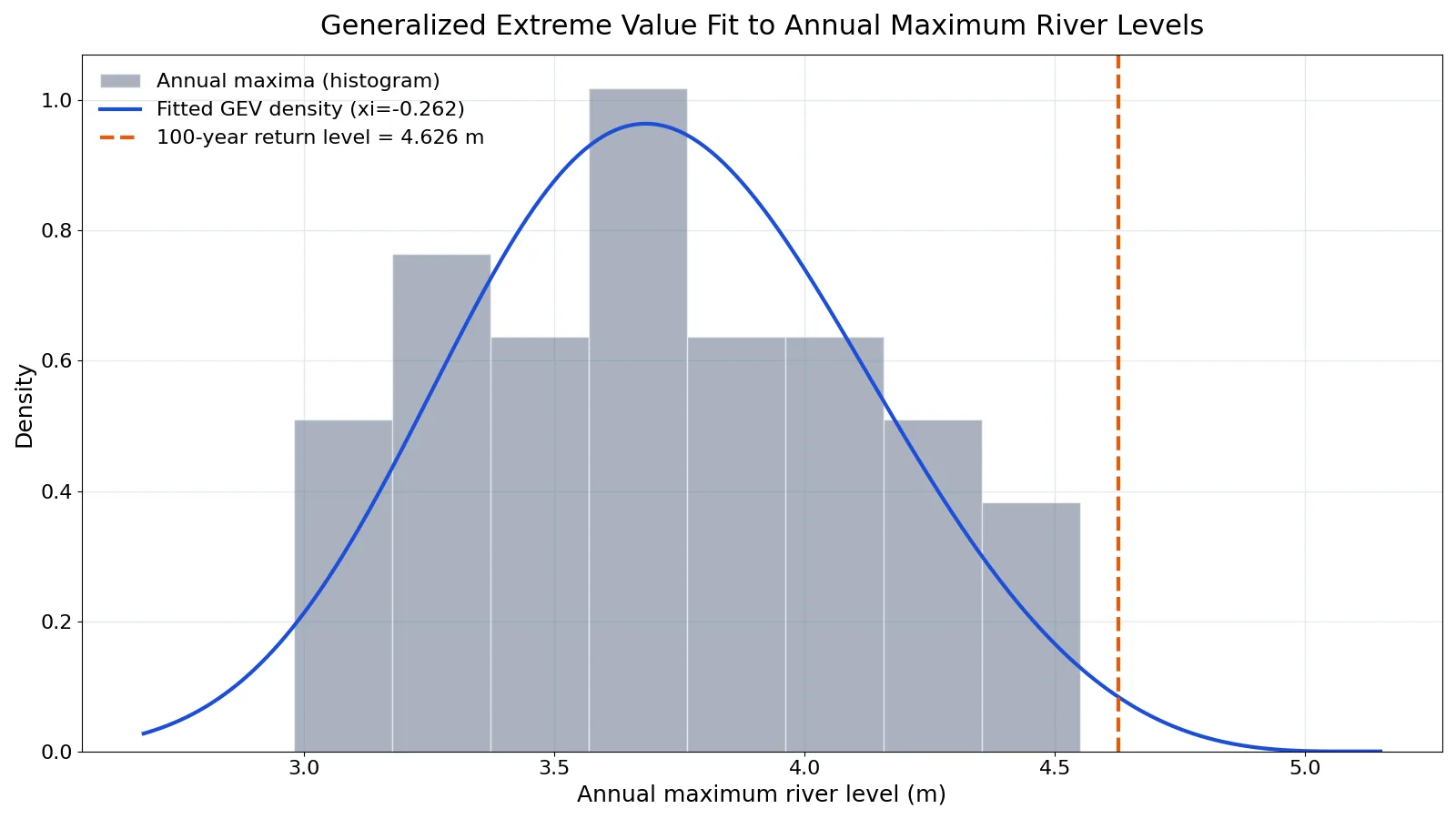
Fitting the GEV by maximum likelihood gives three parameter estimates. The shape parameter is $\xi = -0.2620$, the location is $\mu = 3.5672$ m and the scale is $\sigma = 0.3962$ m. The log-likelihood at the maximum is $-20.5576$. The negative shape estimate means the fitted distribution has a bounded upper tail, so it behaves like the reversed Weibull type.

For a 100-year return period, the non-exceedance probability is $p = 1 - 1/100 = 0.9900$. Inverting the fitted CDF at that probability gives a 100-year return level of $z_{100} = 4.6263$ m. That is the level the model expects to be exceeded once every 100 years on average.

The Python code below fits the same model with SciPy. Note that SciPy's genextreme uses the convention $c = -\xi$, so the sign is flipped when you read the output.

import numpy as np
from scipy import stats
x = np.array([3.12, 3.45, 2.98, 3.67, 4.02, 3.21, 3.88, 4.31, 3.55, 3.09,
              3.74, 4.15, 3.62, 3.28, 4.44, 3.91, 3.33, 3.58, 4.07, 3.19,
              3.85, 4.22, 3.47, 3.71, 4.55, 3.94, 3.36, 3.63, 4.11, 3.24,
              3.79, 4.38, 3.51, 3.68, 4.19, 3.97, 3.42, 3.60, 4.28, 3.15])
c, loc, scale = stats.genextreme.fit(x)
xi = -c
z100 = stats.genextreme.ppf(1 - 1/100, c, loc=loc, scale=scale)
print(f"xi = {xi:.4f}")
print(f"mu = {loc:.4f}")
print(f"sigma = {scale:.4f}")
print(f"100-year return level = {z100:.4f} m")

Output:

xi = -0.2620
mu = 3.5672
sigma = 0.3962
100-year return level = 4.6263 m

How to Interpret It

Read the three parameters together, not one at a time. The location $\mu = 3.5672$ m sits near the middle of the annual maxima, close to the sample mean of 3.7160 m. The scale $\sigma = 0.3962$ m describes how much the annual maxima spread around that center, and it is close to the sample standard deviation of 0.4160 m. The shape $\xi = -0.2620$ tells you the upper tail is bounded, so the fitted curve flattens as you move into the extreme right tail.

The return level is the number most people care about. A 100-year return level of 4.6263 m means the model assigns a 1 percent chance that any given year's maximum exceeds that level. It does not mean the level occurs exactly once per century. It is a probability statement about each block, and the same level can be exceeded twice in a decade or not at all for 200 years.

The shape parameter also tells you how sensitive the return level is to the return period. A negative shape pulls the tail in, so the 100-year level sits closer to the observed maximum of 4.55 m than it would under a heavy-tailed fit. If you compare the fitted density against a histogram of the 40 annual maxima, the curve should follow the bulk of the data and the marked return level should sit to the right of almost every point.

When to Use It (and when not to)

Use the GEV when your data are block maxima and the blocks are large enough that the extreme value limit is a reasonable approximation. Annual maxima of river levels, wind speeds, rainfall or financial losses are the classic cases. The method also suits any setting where you can define equal-length blocks and keep the largest value from each. If you are modeling the minimum instead of the maximum, you can negate the values and fit the same family.

Do not use the GEV on raw data that are not block maxima. If you keep every daily value, the observations are not independent and the extreme value limit does not apply. Do not use it when blocks are too small, because the limiting result needs a large block size to hold. If you want to model values above a high threshold instead of block maxima, the peaks-over-threshold approach is the standard alternative. For general background on how distributions are chosen and compared, see this overview of probability distributions.

Generalized Extreme Value vs Gumbel

The Gumbel distribution is the special case of the GEV with $\xi = 0$. The table below shows how they differ.

Feature	Generalized extreme value	Gumbel
Parameters	Location, scale, shape	Location, scale
Shape parameter	$\xi$ estimated from data	Fixed at $\xi = 0$
Tail behavior	Can be bounded or heavy	Fixed exponential tail
Flexibility	Covers three extreme value types	Covers one type
When to prefer it	You do not know the tail type	You have evidence the tail is Gumbel

The Gumbel is simpler and easier to fit, but it forces the tail to decay at one fixed rate. The GEV lets the data decide, at the cost of one more parameter to estimate. The Gumbel distribution has both minimum and maximum forms, and the maximum form is the one that matches the GEV at zero shape [2]. The Weibull distribution is also connected to this family, since the natural log of Weibull data follows an extreme value distribution [4].

Common Mistakes

Fitting the GEV to raw observations instead of block maxima. The model is built for the maximum of each block, so reduce each block to one value first.
Using blocks that are too short. Small blocks break the extreme value approximation, so prefer annual or longer blocks when you have enough data.
Ignoring the sign convention in software. SciPy's genextreme reports $c = -\xi$, so a reported $c$ of 0.2620 means $\xi = -0.2620$.
Reading a return level as a schedule. A 100-year level is exceeded with 1 percent probability each block, not once per century.
Skipping a goodness-of-fit check. Plot the fitted density against a histogram and check probability plots before trusting return levels.
Forgetting that the shape estimate is uncertain. With only 40 blocks the shape parameter carries wide error bars, so report intervals, not just point estimates.

Limitations

The GEV assumes independent observations within and across blocks. Real maxima often show serial correlation or trends, and ignoring that understates uncertainty in the parameters and return levels. With small samples the shape parameter is hard to pin down, and a small change in $\xi$ can move a long-period return level by a large amount. The model also extrapolates beyond the observed range, so a 100-year level from 40 years of data is an extrapolation that depends heavily on the fitted tail.

The method cannot tell you whether the extreme value limit is appropriate for your data. That is a modeling judgment based on block size and the physical process. If the data have a trend, a regime shift or strong dependence, a stationary GEV will mislead you, and you need a model that accounts for those features.

Frequently Asked Questions

What is the difference between the GEV and the Gumbel distribution?

The Gumbel is the GEV with the shape parameter fixed at zero. The GEV adds a shape parameter that lets the upper tail be bounded or heavy, so it covers three extreme value types instead of one [1]. Use the GEV when you are unsure which tail type fits, and the Gumbel when you have reason to fix the shape at zero.

How much data do I need to fit a GEV?

There is no fixed rule, but block maxima samples are often small because each block yields one value. The example here uses 40 annual maxima, which is enough to estimate the parameters but leaves the shape parameter uncertain. More blocks give tighter estimates, and you should report confidence intervals alongside point estimates.

What does a negative shape parameter mean?

A negative shape parameter means the fitted distribution has a finite upper bound, which is the reversed Weibull type. In the river example, $\xi = -0.2620$ pulls the upper tail in, so the 100-year return level of 4.6263 m sits relatively close to the largest observed value of 4.55 m. A positive shape would give a heavier tail and a larger return level.

How do I compute a return level from a fitted GEV?

Set the probability to $p = 1 - 1/T$ for return period $T$, then invert the fitted CDF at that probability. For the 100-year level, $p = 0.9900$ and the inverted value is 4.6263 m. Most software provides a quantile or percent-point function that does this inversion directly, as shown in the code above.

Can I use the GEV for minima instead of maxima?

Yes. Negate the values, fit the GEV to the negated block minima, then negate the fitted location and the return levels back. The scale and shape keep their fitted values. The same family applies because the minimum of a set of values is the negative of the maximum of the negated values. This keeps you inside one consistent modeling framework.