FV Function in Excel: Future Value Formula and Examples

By Dr. Zubair Khalid, DVM, MS, PhD · 2026-10-03

The Excel FV function returns the future value of an investment or savings plan built from equal periodic payments, a single lump sum, or both. You give it a rate, a number of periods and a payment amount, and it returns the balance at the end of the term. This article covers the fv formula syntax, a full worked example with monthly deposits, and the errors that trip people up.

Quick Answer

FV calculates the value of an investment at a future date, given a constant interest rate and equal payments.
The full syntax is =FV(rate, nper, pmt, [pv], [type]). Only the first three arguments are required.
Money you pay out (deposits) is entered as a negative number. Money you receive (the future value) comes back positive.
For monthly compounding, divide the annual rate by 12 and multiply the years by 12.
The type argument controls timing. Use 0 or omit it for end-of-period payments, use 1 for beginning-of-period payments.

Syntax

Argument	Required?	Meaning
`rate`	Yes	The interest rate per period. For a 6% annual rate compounded monthly, use `0.06/12`.
`nper`	Yes	The total number of payment periods. For 5 years of monthly payments, use `60`.
`pmt`	Yes	The payment made each period. It cannot change over the life of the investment. If omitted, you must supply `pv`.
`pv`	No	The present value, or the lump sum you start with. If omitted, it is assumed to be 0.
`type`	No	When payments are due. `0` means at the end of the period, `1` means at the beginning. If omitted, it is assumed to be 0.

The function returns a single number, the future value. It does not return a schedule of balances, only the ending balance.

How It Works

FV solves the time value of money equation for the ending balance. When you make a series of equal payments at the end of each period, the future value is the sum of every payment grown by compound interest to the final date:

$$FV = pmt \times \frac{(1+rate)^{nper} - 1}{rate}$$

When you also start with a lump sum, that amount grows on its own and is added:

$$FV = pv \times (1+rate)^{nper} + pmt \times \frac{(1+rate)^{nper} - 1}{rate}$$

The sign convention matters. Excel treats cash flowing out as negative and cash flowing in as positive. A deposit of $200 leaves your pocket, so it is entered as -200. The future value that comes back is positive because it is money you would receive.

If you set type to 1, each payment earns one extra period of interest, so the result is larger than the end-of-period case. The type 1 result equals the end-of-period result multiplied by $(1+rate)$.

Worked Example

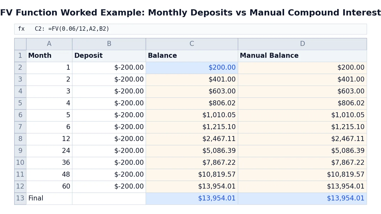
The table below models a savings plan: $200 deposited at the end of every month for up to 60 months, at a 6% annual rate compounded monthly. Column C uses the FV function. Column D uses the manual compound interest formula so you can confirm the two agree.

	A	B	C	D
1	Month	Deposit	Balance	Manual Balance
2	1	-200	`=FV(0.06/12,A2,B2)` -> displays $200.00	`=200*((1+0.06/12)^A2-1)/(0.06/12)` -> displays $200.00
3	2	-200	`=FV(0.06/12,A3,B3)` -> displays $401.00	`=200*((1+0.06/12)^A3-1)/(0.06/12)` -> displays $401.00
4	3	-200	`=FV(0.06/12,A4,B4)` -> displays $603.00	`=200*((1+0.06/12)^A4-1)/(0.06/12)` -> displays $603.00
5	4	-200	`=FV(0.06/12,A5,B5)` -> displays $806.02	`=200*((1+0.06/12)^A5-1)/(0.06/12)` -> displays $806.02
6	5	-200	`=FV(0.06/12,A6,B6)` -> displays $1,010.05	`=200*((1+0.06/12)^A6-1)/(0.06/12)` -> displays $1,010.05
7	6	-200	`=FV(0.06/12,A7,B7)` -> displays $1,215.10	`=200*((1+0.06/12)^A7-1)/(0.06/12)` -> displays $1,215.10
8	12	-200	`=FV(0.06/12,A8,B8)` -> displays $2,467.11	`=200*((1+0.06/12)^A8-1)/(0.06/12)` -> displays $2,467.11
9	24	-200	`=FV(0.06/12,A9,B9)` -> displays $5,086.39	`=200*((1+0.06/12)^A9-1)/(0.06/12)` -> displays $5,086.39
10	36	-200	`=FV(0.06/12,A10,B10)` -> displays $7,867.22	`=200*((1+0.06/12)^A10-1)/(0.06/12)` -> displays $7,867.22
11	48	-200	`=FV(0.06/12,A11,B11)` -> displays $10,819.57	`=200*((1+0.06/12)^A11-1)/(0.06/12)` -> displays $10,819.57
12	60	-200	`=FV(0.06/12,A12,B12)` -> displays $13,954.01	`=200*((1+0.06/12)^A12-1)/(0.06/12)` -> displays $13,954.01
13	Final		`=FV(0.06/12,60,-200)` -> displays $13,954.01	`=200*((1+0.06/12)^60-1)/(0.06/12)` -> displays $13,954.01

Row 13 is the compact version. It skips the helper columns and puts the rate, period count and payment straight into the function. The result, $13,954.01, is the balance after 60 monthly deposits of $200 at 6% compounded monthly. The manual formula in column D returns the same figure, which confirms the FV result.

Notice how the balance grows faster over time. After 12 months you have $2,467.11, which is close to the $2,400 you deposited. By month 60 the balance is $13,954.01 against $12,000 of deposits, so roughly $1,954 of that total is interest earned.

More Examples

A lump sum with no payments. To find what $5,000 grows to in 10 years at 4% compounded annually, leave pmt out and supply pv:

=FV(0.04,10,0,-5000) returns $7,401.22.

Monthly payments with an initial deposit. If you start with $1,000 and add $150 a month for 3 years at 5% compounded monthly:

=FV(0.05/12,36,-150,-1000) returns $6,974.47.

Payments at the beginning of each period. The same 60-month plan with deposits made at the start of each month uses type of 1:

=FV(0.06/12,60,-200,0,1) returns $14,023.78.

That is $69.77 more than the end-of-period version, because every deposit earns one extra month of interest.

Annual instead of monthly. For yearly deposits of $2,000 for 20 years at 5% compounded annually:

=FV(0.05,20,-2000) returns $66,131.91.

If you need to round or adjust these outputs for a report, functions like Excel ROUND handle the formatting step. For a broader tour of what the function library can do, see this overview of Excel functions.

Errors and How to Fix Them

#VALUE! appears when an argument is text instead of a number. Check that rate, nper and pmt are numeric or point to numeric cells.

#NUM! is rare because FV uses a closed-form formula and does not iterate. It can appear when the inputs make the calculation impossible, such as a rate below -1 combined with a fractional nper.

A negative future value is not an error. It means your sign convention is reversed. If you entered deposits as positive numbers, the result flips sign. Enter money paid out as negative.

A result that looks far too large often means the rate was not converted to the period length. A 6% annual rate used directly with monthly periods gives the wrong answer. Divide by 12 for monthly, by 4 for quarterly, by 52 for weekly.

A result that looks far too small usually means nper was entered in years when the rate was monthly. The rate and the period count must use the same time unit.

Common Mistakes

Mixing time units. If rate is monthly, nper must be a count of months. If rate is annual, nper must be a count of years. Fix it by converting both to the same unit before writing the formula.
Forgetting the sign on payments. Deposits are cash out, so they are negative. Entering 200 instead of -200 returns a negative future value. Fix it by adding the minus sign.
Using FV for uneven payments. FV assumes every payment is identical. If your deposits change over time, build a period-by-period schedule instead. The SUM function and its relatives help total those schedules.
Confusing type 0 and 1. The default is end-of-period. If your deposits happen at the start of each month, you must pass 1 or the answer will be slightly low.
Treating the result as exact. FV assumes a constant rate for the whole term. Real accounts change rates, so treat the output as a projection.
Leaving out pv when you have a starting balance. If you already hold money in the account, omitting pv ignores it and understates the result.

Limitations

FV assumes a single fixed interest rate for the entire term and identical payments at regular intervals. Real savings accounts change rates, and real people change how much they deposit. Any result is a projection under those assumptions, not a guarantee. It also ignores fees, taxes and inflation, so the nominal balance it returns is not the same as purchasing power at the end of the term.

The function returns only the ending balance. It does not produce a month-by-month schedule, so you cannot see when the balance crosses a target or how much of each period is interest. For that you need a full amortization or accumulation table, which you can build with the manual formula shown in the worked example. If you need to pull values from a schedule at a variable offset, Excel OFFSET is one way to do it.

Frequently Asked Questions

What does the FV function do in Excel?

FV returns the future value of an investment based on a constant interest rate and equal periodic payments. You supply the rate per period, the number of periods and the payment amount, and it returns the balance at the end of the term. It can also handle a starting lump sum through the pv argument.

Why is my FV result negative?

Excel uses a cash flow sign convention. Money you pay out is negative and money you receive is positive. If your deposits are positive numbers, the function treats them as money coming in and returns a negative future value. Enter deposits as negative numbers to get a positive result.

How do I calculate monthly future value in Excel?

Divide the annual rate by 12 and multiply the number of years by 12. For example, 6% annual compounded monthly becomes 0.06/12, and 5 years becomes 60 periods. Then call =FV(0.06/12,60,-200) for $200 monthly deposits.

What is the difference between type 0 and type 1 in FV?

The type argument sets when payments occur. A value of 0, which is the default, means payments happen at the end of each period. A value of 1 means payments happen at the beginning, so each one earns an extra period of interest and the future value is higher.

Can FV handle a lump sum and regular deposits together?

Yes. Put the starting amount in the pv argument and the recurring amount in pmt. Both must follow the same sign convention. For example, =FV(0.05/12,36,-150,-1000) combines a $1,000 starting balance with $150 monthly deposits.

Does FV account for inflation?

No. FV returns a nominal balance based on the rate you supply. It does not adjust for inflation, taxes or fees. To estimate real purchasing power, subtract an expected inflation rate from your nominal rate before using it in the formula.

References

This article draws on the standard references listed under Further Reading.