What Is a Chi-Square Test? Formula and Examples
By Dr. Zubair Khalid, DVM, MS, PhD ·

A chi square test is a statistical test for categorical data. It compares the counts you actually observed with the counts you would expect if a hypothesis were true, then tells you whether the gap is larger than chance would explain. This article covers the formula, when to use it, and a full worked example.
Quick Answer
- A chi square test works on counts of categories, not on means or continuous measurements.
- The test statistic is $\chi^2 = \sum \frac{(O - E)^2}{E}$, where $O$ is observed and $E$ is expected [1].
- The two main versions are the goodness of fit test (one variable) and the test of independence (two variables in a contingency table) [1][2].
- Degrees of freedom come from the table size, not the sample size. For independence, $df = (r-1)(c-1)$ [3].
- A large chi square value means observed and expected counts are far apart, so the model fits poorly [4].
What Is a Chi Square Test?
A chi square test compares the counts you actually observed in each category with the counts you would expect if nothing unusual were going on, then judges whether the gap is bigger than chance. The formula is χ² = Σ (O - E)² / E, where O is the observed count and E is the expected count in each cell [1]. You square each difference so positive and negative gaps do not cancel, divide by the expected count to weight small and large cells fairly, and add the results across all cells [5].
The test comes in two main versions. A goodness of fit test checks one categorical variable against a theoretical distribution [1]. A test of independence checks whether two categorical variables are related inside a contingency table [1][2]. Both use the same statistic but build expected counts differently. In a goodness of fit test, expected counts come from the theory you are testing [1]. In a test of independence, each expected count is row total times column total divided by the grand total, which is what independence implies [4].
Degrees of freedom come from the table shape, not the sample size. For a table with r rows and c columns, df = (r - 1)(c - 1) [3][4]. A 2x2 table therefore has 1 degree of freedom, a 2x3 table has 2, and a 3x3 table has 4. The answer to the classic multiple choice question is (r - 1)(c - 1), not rc or rc - 1.
Once you have the statistic and the degrees of freedom, you compare the value with the chi square distribution. The distribution is right skewed for small degrees of freedom and becomes more symmetric as degrees of freedom grow [3]. Because every term in the sum is squared, the statistic is never negative, so the test is always right tailed [3]. A large value means observed and expected counts are far apart and the model fits poorly [4].
A small p-value means counts this far from expected would rarely happen under the null, so you reject the null. A large p-value means the data are consistent with the null. The test tells you whether a difference exists, not how big or which direction it runs.
What the Chi Square Test Means
In plain terms, the chi square test asks one question: are the numbers I counted close to the numbers I would expect? If they are close, nothing unusual is happening. If they are far apart, something in the data needs explaining.
The precise definition is narrower. The chi square test is a statistical test that determines whether observed frequencies differ significantly from expected frequencies [5]. You state a null hypothesis of no difference and an alternative hypothesis of a real difference, then reject or fail to reject the null based on the result [5]. The test statistic follows a chi square distribution, which is right skewed for small degrees of freedom and becomes more symmetric as degrees of freedom increase [3]. Because the formula squares each difference, every test statistic is zero or positive, and the test is always right tailed [3].
How It Works
The test statistic is built from one formula applied to every cell:
$$\chi^2 = \sum \frac{(O - E)^2}{E}$$
Each symbol means the following:
- $\chi^2$ is the chi square test statistic, sometimes written as the chi statistic or chi value.
- $O$ is the observed frequency, the count you actually recorded [3].
- $E$ is the expected frequency, the count predicted under the null hypothesis [3].
- $\sum$ means sum across all cells in the table.
For each cell you subtract the expected count from the observed count, square the difference, and divide by the expected count. Then you add those values across all cells [5]. A large sum means the observed and expected values are not close and the model is a poor fit [4].
Expected counts depend on the test. In a goodness of fit test, expected counts come from a theoretical distribution [1]. In a test of independence, the expected count for a cell is the row total times the column total divided by the grand total, because that is what independence implies [4].
Degrees of freedom also depend on the test. For a two-way table with $r$ rows and $c$ columns, the degrees of freedom are:
$$df = (r-1)(c-1)$$
This follows from the table having $rc$ cells with one determined by the others, and from estimating $(r-1) + (c-1)$ marginal parameters under independence [4][3].
Worked Example
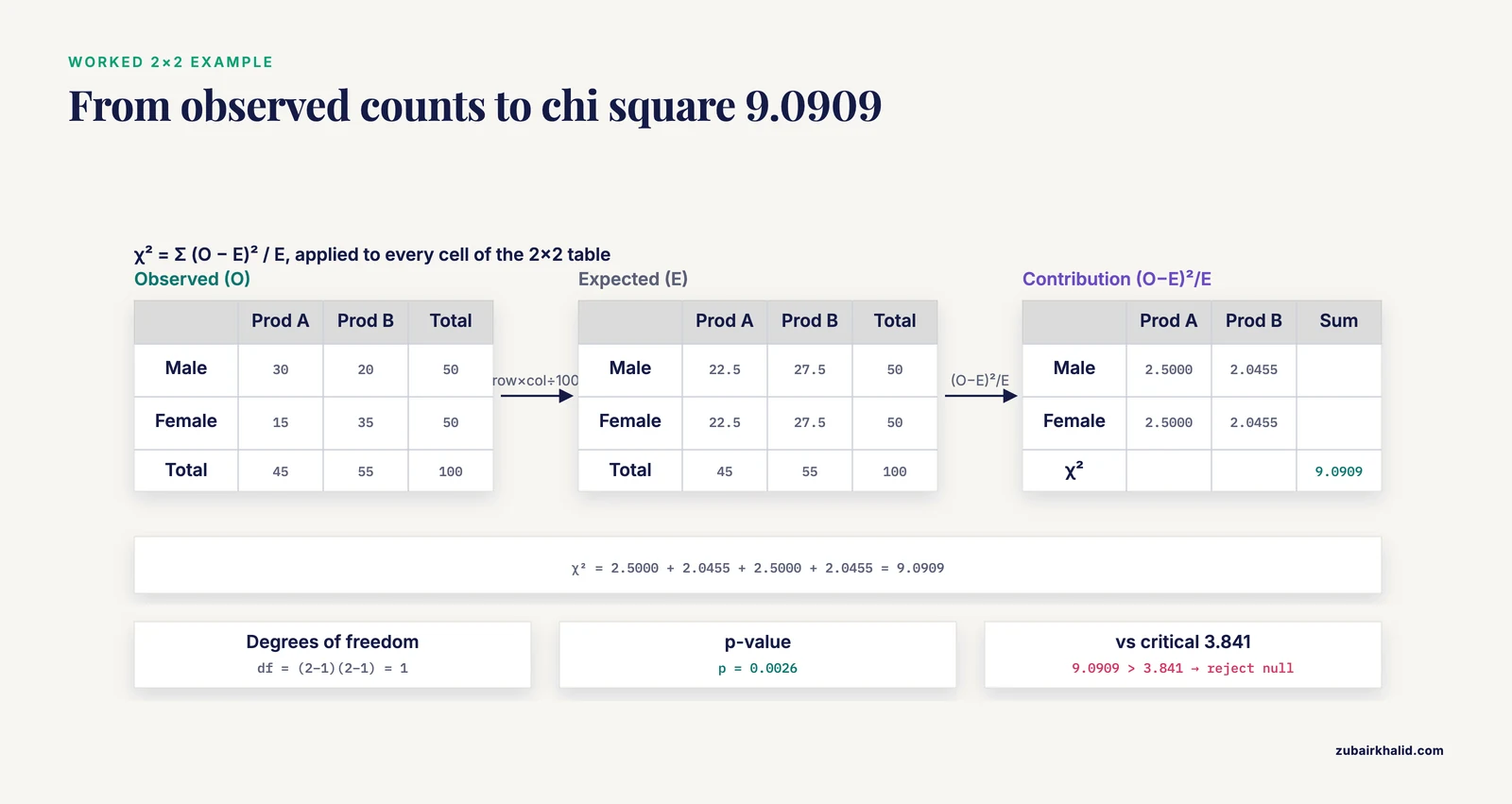
A survey of 100 respondents recorded gender and product preference. The data are counts of people in each combination.
| Gender | Preference | Count |
|---|---|---|
| Male | Product A | 30 |
| Male | Product B | 20 |
| Female | Product A | 15 |
| Female | Product B | 35 |
Arranged as a 2x2 table with rows for gender and columns for preference, the observed counts are:
| Product A | Product B | Row total | |
|---|---|---|---|
| Male | 30 | 20 | 50 |
| Female | 15 | 35 | 50 |
| Column total | 45 | 55 | 100 |
The row totals are 50 and 50, the column totals are 45 and 55, and the grand total is 100.
Expected counts use row total times column total divided by the grand total. Every cell works out the same way here because both row totals are 50:
| Product A | Product B | |
|---|---|---|
| Male | 22.5000 | 27.5000 |
| Female | 22.5000 | 27.5000 |
Now compute each cell contribution:
- Male, Product A: $(30 - 22.5000)^2 / 22.5000 = 2.5000$
- Male, Product B: $(20 - 27.5000)^2 / 27.5000 = 2.0455$
- Female, Product A: $(15 - 22.5000)^2 / 22.5000 = 2.5000$
- Female, Product B: $(35 - 27.5000)^2 / 27.5000 = 2.0455$
Summing the four contributions gives a chi square statistic of 9.0909. The degrees of freedom are $(2-1)(2-1) = 1$. The p-value is 0.0026.
You can reproduce this in Python:
import numpy as np
from scipy.stats import chi2_contingency
obs = np.array([[30, 20], [15, 35]])
chi2, p, dof, exp = chi2_contingency(obs, correction=False)
print(chi2, p, dof, exp)
Output:
9.09090909090909 0.0025688315270227164 1 [[22.5 27.5]
[22.5 27.5]]If you want to run your own numbers without writing code, the chi square test calculator takes a contingency table and returns the statistic, degrees of freedom, and p-value.
How to Interpret It
Start with the p-value. It answers a specific question: if the null hypothesis were true, how often would you see a chi square value at least this large? A small p-value means the observed counts are unlikely under the null.
In the example, the p-value is 0.0026. At a 0.05 significance level you reject the null hypothesis of independence. Gender and product preference appear to be associated in this sample.
Compare the statistic with a critical value if you prefer that route. The critical value for a chi square distribution with 1 degree of freedom at the 0.05 level is 3.841, so the calculated value of 9.0909 here exceeds it and leads to rejecting the null. You can look up these thresholds in a chi square table of critical values.
A significant result tells you that an association exists. It does not tell you which cells drive it. For that you need post-hoc work such as standardized residuals and partitioning.
When to Use It (and when not to)
Use a chi square test when your data are counts of categories and you want to compare those counts with expectations. The three standard uses are comparing observed and expected frequency distributions of a nominal variable, testing whether two variables are independent, and using the chi square distribution in work on correlation coefficients [2].
Typical research questions look like this. Does the distribution of eye colors at a university differ from the general population? Do kindergarten students prefer ice cream flavors equally? [6] Both are count comparisons against an expectation.
Do not use a chi square test for continuous measurements such as height or reaction time. Group continuous data into intervals first if you must, though the choice of intervals affects the power of the test [7]. Do not use it when expected counts are very small. A common rule of thumb requires an expected count of at least five in every cell [7]. When a 2x2 table has small expected counts, a Fisher exact test is usually the better choice.
Chi Square Test vs t-Test
The closest related idea is the t-test, which compares means. The two tests answer different questions about different data types.
| Feature | Chi square test | t-test |
|---|---|---|
| Data type | Counts of categories | Continuous measurements |
| Compares | Observed vs expected frequencies | Means of two groups |
| Null hypothesis | No association or no difference from expected | No difference in means |
| Test statistic | $\chi^2 = \sum (O-E)^2/E$ | Based on difference in means over standard error |
| Distribution | Chi square, right tailed | t distribution, symmetric |
If your outcome is a category count, use chi square. If your outcome is a numeric average, use a two sample t-test. For comparing two proportions directly, a two proportion z-test is another option.
Common Mistakes
- Using raw counts where percentages belong, or the reverse. The formula needs frequencies, not proportions. Convert percentages back to counts before computing.
- Computing expected counts incorrectly. For independence, each expected count is row total times column total divided by grand total [4]. Do not divide by the number of cells.
- Getting degrees of freedom wrong. Use $(r-1)(c-1)$ for a contingency table [3], not the number of cells and not the sample size.
- Ignoring small expected counts. If any expected count is below about five, the chi square approximation is unreliable [7]. Combine categories or switch to an exact test.
- Treating a significant result as proof of causation. The test detects association. It says nothing about which variable causes the other.
- Running the test on paired data. Chi square assumes independent observations. Repeated measures on the same subjects need a different method.
Limitations
The chi square test only detects departures from the null. It cannot tell you the size or direction of an effect, and a significant result in a large sample may reflect a trivial difference. Report the counts alongside the statistic so readers can judge practical relevance.
The test is also sensitive to how you define your categories. For goodness of fit tests on continuous data, the number of groups and how group membership is defined affect the power of the test, and only rules of thumb exist for choosing them [7]. Results can shift when you redraw the boundaries.
The Formula Step by Step
The chi square formula looks compact, but each piece has a job. Walking through it cell by cell removes most confusion.
What each symbol does
O is the observed frequency, the count you recorded [3]. E is the expected frequency, the count predicted under the null hypothesis [3]. The subtraction O - E gives the raw gap. Squaring it makes every gap positive, so a cell with too many observations and a cell with too few both count as misfits. Dividing by E scales the gap to the size of the cell, so a gap of 5 matters more when 10 were expected than when 1,000 were expected. The sigma sign adds these scaled gaps across every cell [5].
Why the statistic is always positive
Because each term is a square, no cell can contribute a negative amount. The smallest possible value is 0, which happens only when every observed count equals its expected count exactly. This is why the test is one tailed: you only care whether the misfit is unusually large, never unusually small [3].
Reading the result
A large sum means the observed and expected values are not close and the model is a poor fit [4]. You then convert that sum to a p-value using the chi square distribution with the correct degrees of freedom. The p-value answers one question: if the null were true, how often would a statistic at least this large appear?
A Goodness of Fit Example
The independence test is covered in the main article. A goodness of fit test uses the same formula but a different source of expected counts, and it is worth seeing side by side.
Suppose a candy bag is advertised as containing equal numbers of four colors, and you count 100 candies. Under the advertised claim, each color should appear 25 times. Your observed counts are 34, 22, 19, and 25.
Each contribution is (O - 25)² / 25. For the four cells these are 3.24, 0.36, 1.44, and 0.00. The sum is 5.04. With four categories and one fixed total, df = 4 - 1 = 3. You then compare 5.04 against the chi square distribution with 3 degrees of freedom.
Notice the difference from the independence test. Here the expected counts came from a stated theory, not from row and column totals [1]. The degrees of freedom also differ: a one variable table with k categories gives k - 1, while a two variable table gives (r - 1)(c - 1) [3][4]. Mixing up these two rules is one of the most common errors.
The same caution about small expected counts applies. If any expected count falls below about five, the approximation is unreliable and you should combine categories or use an exact method [7].
Degrees of Freedom in Words
Picture the contingency table as a grid of locked cells. Once the row totals and column totals are fixed, you can fill in most cells freely, but the last cell in each row and each column is forced, because it must make the total come out right.
In a 2x2 table, fixing the margins leaves exactly one cell free. Fill that one and the other three are determined. That is why df = 1. In a 3x3 table, two cells in the first row and two in the first column can vary, and the rest follow, giving 4. The general count is (r - 1)(c - 1) [3][4].
This is also why the degrees of freedom do not depend on how many people you surveyed. A 2x2 table with 40 respondents and a 2x2 table with 4,000 respondents both have 1 degree of freedom. Sample size affects the p-value, not the df.
Common Misconceptions
"A big chi square always means the variables are related"
It means the counts depart from the expected pattern. In a very large sample, a trivial departure can produce a large statistic and a small p-value. Always report the counts so readers can judge whether the departure matters in practice.
"The test proves causation"
It detects association only. It cannot tell you which variable drives the other, or whether a third variable explains both.
"You can use it on averages"
No. The test works on counts of categories [2]. Continuous measurements such as height or reaction time need a different test, such as a t-test, unless you first group them into intervals, and the choice of intervals affects the power of the test [7].
"Small expected counts are fine if the total is large"
The rule of thumb is about each cell, not the grand total. An expected count below about five in any cell makes the approximation unreliable [7]. Combine sparse categories or switch to an exact test.
"The degrees of freedom are the number of cells"
Use (r - 1)(c - 1) for a contingency table [3], and k - 1 for a one variable goodness of fit table. Neither equals the number of cells.
Frequently Asked Questions
What is the difference between a chi square test and a chi square distribution?
The distribution is the probability curve the statistic follows. The test is the procedure that produces a statistic and compares it against that curve. The distribution is right skewed for small degrees of freedom and becomes more symmetric as degrees of freedom increase [3]. You can read more about the shape and its properties in this guide to the chi square distribution.
What does a chi square value of 0 mean?
A value of 0 means every observed count exactly equals its expected count. There is no deviation at all. In practice this almost never happens with real data, and a value near 0 simply indicates a very close fit.
Can I use a chi square test with only two categories?
Yes. A 2x2 table is the most common setup, and it gives 1 degree of freedom. The example in this article uses exactly that design. Just check that all expected counts are large enough for the approximation to hold.
How many observations do I need for a chi square test?
There is no fixed sample size rule. What matters is the expected count in each cell. A common rule of thumb requires an expected count of at least five in every cell [7]. If your expected counts fall below that, combine categories or use an exact test.
What is the difference between the goodness of fit test and the test of independence?
The goodness of fit test compares one variable's observed frequencies against a theoretical distribution [1]. The test of independence checks whether two categorical variables are associated in a contingency table [1]. Both use the same statistic, but they differ in how expected counts are derived.
References
- 11: Chi-Square Test - Statistics LibreTexts
- Witt PL, McGrain P. Witt PL, McGrain P. (1986). Nonparametric testing using the chi-square distribution. Physical therapy
- 10.1: Chi-Square Test for Independence - Mathematics LibreTexts/10%3A_Goodness_of_Fit_and_Test_for_Independence/10.01%3A_Chi-Square_Test_for_Independence)
- Chi-Square Goodness of Fit Test
- CHI-SQUARE
- Chi-Square Tests - Statistics Resources - LibGuides at National University
- 7.2.1.1. Chi-square goodness-of-fit test
Related Articles
- Chi-Square Distribution: Definition, Formula and Examples
- Two Sample t-Test: Formula, Calculation and Example
- Chi-Square Table: How to Read It and Find Critical Values
- Two Proportion Z-Test: Formula and Worked Example
- Excel ROUND Function: Formula and Examples
- Genetics lab report example chi-square
- Post-Hoc Tests After a Significant Chi-Square
- Chi-Square Test of Independence vs. Fisher