How to Validate Your Bioinformatics Analysis
By Dr. Zubair Khalid, DVM, MS, PhD ·

By the end of this article you will be able to validate bioinformatics analysis results in four layers: data and quality-control checks, internal statistical validation, external validation on independent cohorts, and orthogonal confirmation with a second measurement technology. You will run a receiver operating characteristic (ROC) analysis, a cross-validated model, and a label-permutation test, and you will know how to catch the leakage errors that quietly invalidate many published pipelines.
To follow the walkthrough you need a computer with at least 8 GB of RAM, R version 4.2 or newer, Python 3.10 or newer, the conda package manager, and Git. Everything runs on a laptop. No sequencing data of your own is required, because public repositories such as the Gene Expression Omnibus (GEO) provide the test datasets.
What Validation Means in Bioinformatics
Validation answers one question: would this result survive contact with data your analysis never saw? An analysis that only reproduces patterns inside its own training data has not been validated. It has been described.
Current bioinformatics papers show what a layered validation looks like in practice. A study of depression and influenza A virus infection combined Mendelian randomization, differential expression, protein-protein interaction (PPI) analysis, ROC curve validation on external datasets, single-cell RNA sequencing, virtual knockout simulation, molecular docking, and finally in vitro experiments in influenza-infected Jurkat T cells [1]. A lung cancer microRNA signature study carried its nine-miRNA panel from TCGA tissue data through machine-learning feature selection, three independent public cohorts, and then RT-qPCR in an institutional serum cohort of 259 participants [2]. A forensic toxicology study of acute myocardial ischemia in mice screened biomarkers with weighted gene co-expression network analysis (WGCNA) and least absolute shrinkage and selection operator (LASSO) regression, evaluated them with ROC curves, and then confirmed expression by real-time quantitative PCR in an actual mouse model [3].
Notice the pattern. None of these studies treats a single statistic as proof. Each one asks a slightly different question with a different data source, a different method, or a different measurement platform, and looks for agreement. That agreement is validation.
The rest of this article turns that pattern into a procedure you can execute.
The Four Layers of Validation
Layer 1: Data and Quality Control
Before any statistics, confirm the inputs are real. This means checking read quality with FastQC or a similar tool, confirming sample metadata matches the experimental design, verifying that group labels have not been swapped, and checking that gene or protein identifiers map to a consistent reference. A surprising number of failed replications trace back to a mislabeled column or an unannounced batch effect, not to the model.
Identifier mapping deserves special attention. The same metabolite or gene can carry different IDs in KEGG, PubChem, Ensembl, and Entrez Gene. Tools such as MetaMapR handle this by routing identifiers through a Chemical Translation System that converts between more than 200 common biochemical databases, which is the level of care identifier conversion needs before you trust any downstream intersection [4].
Layer 2: Internal Statistical Validation
Internal validation asks whether the result is stable within the dataset you have. The two workhorse methods are resampling and discrimination metrics. Cross-validation repeatedly splits your data, fits the model on one part, and tests on the other. ROC analysis, quantified as the area under the curve (AUC), asks how well a score separates the two classes. An AUC of 0.5 is chance and an AUC of 1.0 is perfect separation.
The critical internal test is the gap between the apparent performance (measured on the data used to fit the model) and the cross-validated performance. A model whose apparent AUC is 0.95 and whose cross-validated AUC is 0.62 has memorized its training samples. That gap is the single most informative number in any validation report, and most published overclaims trace back to it being hidden or never computed.
Layer 3: External Validation
External validation means locking your entire pipeline (feature selection included) and applying it, unchanged, to a dataset you never touched during development. The lung cancer miRNA study did exactly this, designating GSE188232 as the development dataset, GSE211692 as a cross-dataset evaluation cohort, and GSE137140 as an additional histologically annotated serum cohort, then reporting performance across age, sex, stage, nodal, and metastatic subgroups [2].
External validation is stricter than cross-validation because the new cohort usually comes from a different laboratory, platform, or population. Performance almost always drops on external data. A modest drop (for example, from an AUC of 0.90 to 0.80) is normal and still meaningful. A collapse to near 0.5 tells you the original signal was dataset-specific.
Layer 4: Orthogonal and Experimental Validation
The strongest layer confirms the finding with a technology that does not share the biases of the original. For transcriptomics this is usually RT-qPCR on independent biological samples, ideally with the same direction of change and a comparable effect size. The mouse ischemia study validated its top biomarker this way, reporting an AUC of 0.91 for IκBα, 0.78 for BTG2, and 0.77 for USE1, then confirming expression differences across control, ischemia, and acute ischemia groups by qPCR [3]. The ovarian aging study validated BAG2, BLVRB, and PHB2 downregulation by RT-qPCR, providing a cautionary example as well, because the fourth candidate, STC1, did not reach significance in the experimental confirmation [5]. Functional confirmation can go further, as in the in vitro Jurkat T cell infection experiments used to test the depression-influenza key gene and its candidate compound [1].
Step-by-Step Walkthrough: Validating a Diagnostic Gene Signature
This walkthrough uses a common design: discover a small gene signature that separates disease from control, then validate it honestly. The commands are real. Numeric outputs are illustrative unless tied to a cited study, so run them on your own data and interpret your own values.
Step 1: Build a Reproducible Environment
Validation is impossible to audit if nobody can recreate your software versions. Start with a pinned environment and version control.
conda create -n validate -y -c conda-forge r-base=4.3 python=3.11
conda activate validate
Rscript -e 'install.packages(c("GEOquery","limma","pROC","caret","sva"))'
git init validate-project
Then record the environment inside every analysis script.
set.seed(42)
cat(R.version.string, "\n")
packageVersion("limma")
packageVersion("pROC")
Expected output looks like this:
R version 4.3.2 (2023-10-31)
[1] '1.52.0'
[1] '1.18.0'
Save the full sessionInfo() output to a text file at the end of every script. A reviewer or collaborator should be able to reinstall that exact world and rerun your analysis from raw data to figure.
Step 2: Download and Inspect the Data
Download a public GEO series and inspect it before analyzing anything.
library(GEOquery)
gse <- getGEO("GSE126848", GSEMatrix = TRUE)
exprs_df <- exprs(gse[[1]])
pdata <- pData(gse[[1]])
dim(exprs_df)
table(pdata$`disease status:ch1`)
Expected output:
[1] 46257    57
     control       MASH
        26         31
Now verify three things. First, do the group counts match what the paper reports? Second, are there duplicated samples or duplicated patient IDs? Third, do the expression distributions look comparable between groups, or does one group sit visibly higher (a classic batch signature)? This dataset pairs a MASH group with controls in a published neuroinflammation biomarker study, which makes it a useful test case because that study openly discusses the limits of its own validation design [6].
Step 3: Re-Derive the Primary Result
Fit the primary differential expression model with limma, using an empirical Bayes moderated test and Benjamini-Hochberg correction for multiple testing.
library(limma)
group <- factor(pdata$`disease status:ch1`,
                levels = c("control", "MASH"))
design <- model.matrix(~ group)
fit <- lmFit(exprs_df, design)
fit <- eBayes(fit)
deg <- topTable(fit, coef = 2, number = Inf, adjust.method = "BH")
sig <- subset(deg, adj.P.Val < 0.05 & abs(logFC) > 1)
nrow(sig)
head(sig, 5)
Expected output shape:
[1] 1243
            logFC  AveExpr     t  P.Value adj.P.Val     B
GENE1        1.31     8.10  6.42  2.1e-09   3.0e-07  13.4
GENE2       -1.12     6.55 -5.90  9.8e-09   6.1e-07  11.8
The sanity checks here are quantitative. A differential expression analysis of human tissue typically yields on the order of hundreds to a few thousand significant genes under these thresholds. If you get 12 genes or 40,000, suspect a design matrix error, swapped labels, or unnormalized data. Also check the sign convention: in model.matrix(~ group) with control as the reference, a positive logFC means up in disease. Getting this backward is one of the most frequent silent errors in reanalysis projects.
Step 4: ROC Validation With a Worked Calculation
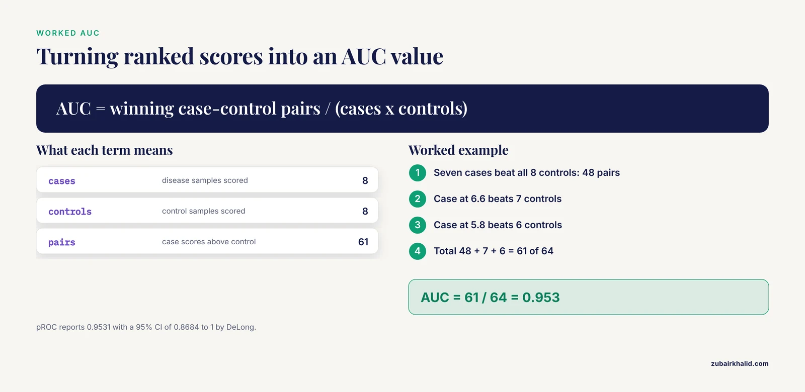
Suppose your pipeline has selected a single gene score and you want to know how well it separates 8 cases from 8 controls. This toy dataset keeps the arithmetic visible.
Cases: 9.1, 8.7, 8.2, 7.9, 7.4, 7.0, 6.6, 5.8 Controls: 6.9, 6.2, 5.5, 5.1, 4.8, 4.4, 3.9, 3.1
The AUC equals the Mann-Whitney U statistic divided by the product of the group sizes. Count every case-control pair where the case scores higher. Seven cases beat all 8 controls, the case at 6.6 beats 7 controls, and the case at 5.8 beats 6 controls, giving 48 + 7 + 6 = 61 winning pairs out of 8 × 8 = 64 possible pairs.
AUC = 61 / 64 = 0.953
Confirm with pROC and get a confidence interval:
library(pROC)
scores <- c(9.1, 8.7, 8.2, 7.9, 7.4, 7.0, 6.6, 5.8,
            6.9, 6.2, 5.5, 5.1, 4.8, 4.4, 3.9, 3.1)
status <- factor(c(rep("case", 8), rep("control", 8)),
                 levels = c("control", "case"))
roc_fit <- roc(status, scores, direction = "<", quiet = TRUE)
auc(roc_fit)
ci.auc(roc_fit)
Expected output:
Area under the curve: 0.9531
95% CI: 0.8684-1 (DeLong)
Report AUC with a confidence interval, never as a bare point estimate. For context on what published biomarker studies report, the myocardial ischemia study considered an AUC of 0.78 (BTG2) acceptable for a secondary biomarker and reserved its strongest claim (AUC 0.91) for the top marker [3], while the ovarian aging study reported per-gene AUCs between 0.73 and 0.77 in the discovery dataset [5]. Diagnostic AUCs in the 0.7 to 0.8 range are commonly called moderate, 0.8 to 0.9 good, and above 0.9 excellent, but the thresholds are conventions, not laws. What matters more is how much performance survives external validation.
Step 5: Cross-Validate the Full Pipeline
The crucial rule is that feature selection must happen inside the cross-validation loop. Selecting features on all data and then cross-validating the classifier leaks information and inflates every metric.
library(caret)
set.seed(42)
ctrl <- trainControl(method = "cv", number = 10,
                     classProbs = TRUE,
                     summaryFunction = twoClassSummary)
model <- train(x = X, y = status,
               method = "glm",
               trControl = ctrl,
               metric = "ROC")
model
Expected output shape:
Resampling results across 10-fold cross-validation:

  ROC       Sens   Spec
  0.81      0.75   0.72
Compare this cross-validated ROC against the apparent AUC from Step 4. If the apparent value is 0.95 and cross-validation gives 0.81, that gap is honest information about generalization. If the cross-validated value lands at 0.52, the signature does not exist as a multivariable model even if individual genes looked promising.
Step 6: External Validation on an Independent Cohort
Freeze every choice (gene list, coefficients, cutoffs, direction) and apply them to a second dataset, downloaded separately and never opened during development.
gse2 <- getGEO("GSE89632", GSEMatrix = TRUE)
exprs2 <- exprs(gse2[[1]])
pd2 <- pData(gse2[[1]])

# Apply the locked signature. No re-selection, no refitting.
locked_score <- colMeans(exprs2[sig_genes, , drop = FALSE])
new_status <- factor(pd2$`disease status:ch1`,
                     levels = c("control", "MASH"))
roc_ext <- roc(new_status, locked_score,
               direction = "<", quiet = TRUE)
auc(roc_ext)
Expected output shape:
Area under the curve: 0.78Interpret the drop, not just the number. Going from an internal AUC of 0.81 to an external AUC of 0.78 is a strong result. Going from 0.95 to 0.55 means the signature was an artifact of the development cohort. Also check whether the genes keep the same direction of effect in the external set, because a reversed sign is a red flag for batch confounding or a mislabeled group.
The miRNA signature study illustrates the full spectrum of external checking: separate evaluation cohorts for cross-dataset performance, a histologically annotated serum cohort for subgroup analysis across age, sex, and stage, and finally institutional RT-qPCR confirmation in 259 participants [2]. You do not need all of those layers, but the more you add, the fewer alternative explanations remain.
Step 7: Sensitivity Analyses and Negative Controls
Run the analyses that could falsify your result.
First, a label permutation test. Shuffle the case-control labels 1,000 times and recompute the AUC each time. Real signal produces permuted AUCs centered near 0.5, and your observed AUC should sit far in the tail.
perm_auc <- replicate(1000, {
  perm <- sample(status)
  as.numeric(auc(roc(perm, scores, direction = "<",
                     quiet = TRUE)))
})
mean(perm_auc >= 0.9531)
Expected output:
[1] 0A p-value of 0 here means none of 1,000 random labelings matched your observed AUC. If hundreds of permutations match your result, the signal is noise.
Second, test batch sensitivity. Regress known batch variables out of the expression matrix with limma::removeBatchEffect, rerun the analysis, and check that the same genes remain significant. If your signature disappears after batch correction, it was measuring the processing batch, not biology.
Third, check method robustness. If your finding only appears with one feature-selection method, that is weak. The ischemia study triangulated with WGCNA, LASSO, and ROC curves rather than trusting a single algorithm [3], and methods tutorials that compare seven Bayesian multi-study factor models plus two benchmark approaches through extensive simulations make the same point systematically: conclusions should not hinge on one implementation choice [7].
Fourth, check identifier robustness. Rebuild your gene list from a second annotation source and confirm the intersection is stable. If your 24 overlapping DEGs [1] become 9 with a different annotation build, every downstream module depends on an unstable foundation.
Step 8: Orthogonal Experimental Validation
For a transcriptomic claim, RT-qPCR on independent samples is the standard first orthogonal check. Validate at least the top candidates, not all of them, and pre-specify the direction you expect. The ovarian aging study did this honestly, confirming three of four key genes by RT-qPCR and reporting the fourth as not significant rather than quietly dropping it [5]. That transparent discordance is more informative for readers than four clean confirmations, because it bounds the reliability of the computational screen.
If the resources exist, functional validation closes the loop: in vitro infection experiments [1], an actual mouse ischemia model [3], or in vitro testing of the two hub genes identified by Random Forest in the endothelial-to-mesenchymal transition study, where CCL5 and IL1B showed individual diagnostic AUCs above 0.7 that rose above 0.85 in a combined model [8].
Validation Checklist
| Check | Tool or command | What a pass looks like |
|---|---|---|
| Environment pinned | sessionInfo(), Git commit hash | Exact package versions recorded, raw data archived |
| Input data verified | dim(), table(group) | Group counts match the published design, no duplicate IDs |
| DE result sane | nrow(sig) | Result count in the expected range, logFC signs correct |
| Discrimination | pROC::auc, ci.auc | AUC reported with a 95% confidence interval |
| Overfitting check | 10-fold CV inside feature selection | CV AUC close to apparent AUC |
| Label permutation | 1,000 shuffled labels | Observed AUC far outside the permutation distribution |
| External cohort | Locked model on new GEO accession | Direction of effect preserved, modest AUC drop |
| Batch sensitivity | removeBatchEffect | Signature survives correction |
| Orthogonal assay | RT-qPCR, independent samples | Same direction of change, candidates pre-specified |
| Full audit trail | Script + sessionInfo | A stranger can rerun the analysis end to end |
Common Mistakes and Limitations
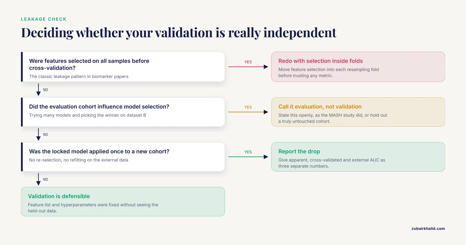
These are the errors that most often invalidate bioinformatics results, in rough order of frequency.
Using the evaluation cohort during model selection. If you try many candidate models and pick the winner using dataset B, then report dataset B as validation, you have not validated anything. One MASH biomarker study stated this explicitly, noting that because its evaluation set contributed to model selection it did not represent a fully independent validation cohort [6]. That sentence is a model of honest reporting. Most papers never write it, and most readers never notice.
Screening 100 model combinations and reporting the best as if it were pre-specified. The same study evaluated 113 machine learning algorithm combinations and moved forward with 81 [6]. With that many candidates, some will look excellent on any dataset by chance alone. Correct the search: either pre-specify one model, or use nested cross-validation so the model-selection step happens inside each resampling fold, or hold out a truly untouched external cohort evaluated exactly once.
Selecting features before cross-validation. This is the most common leakage pattern in biomarker papers. Differentially expressed genes are chosen on all samples, then a classifier on those genes is cross-validated. The CV folds are not independent because the feature list already saw every label. The fix costs nothing: move feature selection inside each fold.
Building an ROC curve on the data that selected the gene. A gene chosen for being differentially expressed will trivially discriminate in the discovery set. The AUC that matters is computed on samples that played no role in choosing the gene, ideally in a different laboratory.
Treating descriptive analyses as validation. A PPI network, a GO enrichment plot, and an immune infiltration estimate re-express your gene list in different vocabularies. They can generate hypotheses but they do not confirm it, because they share the same input. True validation requires either new data or a new measurement technology. The strongest published pipelines layer both, pairing computational screens with ROC checks on external datasets and then qPCR or cell experiments [1], [3].
Ignoring platform and preprocessing differences between cohorts. Before merging or comparing datasets, confirm the annotation versions, normalization, and log transformation are compatible. Reference-guided preprocessing decisions, such as extracting a target sequence from full-genome assemblies via MAFFT alignment before comparison, materially change downstream results and must be documented in the methods [9].
Expecting perfect concordance from orthogonal validation. Some candidates will fail qPCR or functional testing. Three of four genes confirmed in one ovarian aging study [5] is a normal outcome, not a failed study. Plan the candidate list and the write-up for partial confirmation.
Skipping negative controls. Permute your labels, scramble your gene lists, and analyze a random equal-sized gene set. If your real result does not clearly beat its own negative controls, no amount of downstream plot-making will fix it.
Reproducibility gaps. No random seed, no sessionInfo(), no archived raw data, and an analysis that only runs on one laptop in one order. A validation claim is only as strong as the audit trail behind it.
One general limitation applies to everything above. The right validation design depends on your specific question, data type, and sample size, and a consulting statistician or senior bioinformatician can review your plan in an hour and save you months. Budget for that conversation before the analysis, not after.
How to Report Validation So Others Can Trust It
A validation report should let a reader answer four questions without emailing you. What was locked before external testing? What was re-estimated? What were the exact data accessions? What software versions and seeds produced the numbers?
Concretely, report the apparent AUC, the cross-validated AUC, and the external AUC as three separate numbers, with confidence intervals on each. State which dataset served which role, following the explicit dev/evaluation/validation split used in the miRNA signature work [2]. State clearly when an evaluation cohort influenced model selection, as the MASH study did [6]. List preprocessing steps in order, including alignment and annotation versions as end-to-end virology pipelines do [9]. Deposit the code, the session information, and the locked feature list. If a computational framework paper can publish 2,502 sequences processed through a documented pipeline from raw GenBank retrieval through embedding-space analysis, your gene signature study can publish its ten-line preprocessing block.
Building Your Validation Skills
Validation is a learnable skill, and the fastest route is executing other people's analyses until the failure modes feel familiar. For network methods, Graphery provides interactive tutorials that pair each graph concept with executable Python code you can modify and run on real biological networks without an account [10]. For microbiome work, the PUMAA curriculum teaches undergraduate-level analysis, visualization, and statistical reasoning on targeted amplicon data while deliberately avoiding a steep command-line barrier [11]. A structured bioinformatics course that forces you to complete a full project with a held-out test set will teach validation faster than reading about it, because you will watch your own cross-validated AUC drop below your apparent AUC and have to explain why. The R and Python packages used throughout this walkthrough, including limma, pROC, caret, and GEOquery, are the standard toolset for this skill set, and practicing on public GEO data removes every excuse about missing samples.
Frequently Asked Questions
What does it mean to validate bioinformatics analysis results?
It means demonstrating that your findings hold under conditions your analysis did not control: new samples, new methods, new measurement platforms, and deliberately corrupted inputs. Validation has four layers, data quality checks, internal statistical testing, external cohort testing, and orthogonal experimental confirmation, and a claim becomes credible as it survives more layers.
How do I validate bioinformatics analysis results step by step?
Pin your software environment, verify raw data and group labels, re-derive the primary result with sanity checks, compute ROC or discrimination metrics with confidence intervals, cross-validate the entire pipeline including feature selection, test a locked model on an independent cohort, run permutation and batch-sensitivity checks, and confirm key findings with RT-qPCR or a functional assay.
Is a cross-validated AUC enough, or do I need external validation?
Cross-validation alone is not enough when the external data come from a different laboratory, platform, or population, because cross-validation shares preprocessing and population with your training data. If your goal is a diagnostic claim or any statement about samples outside your cohort, you need at least one truly independent dataset evaluated once with a locked pipeline.
Why did my AUC drop on the external dataset?
Performance almost always drops on external data because batch effects, population differences, and platform noise add variance the model never saw. A drop from 0.90 to 0.78 is usually fine. A drop to 0.55 means the original signal was specific to the development cohort, most often through feature-selection leakage or batch confounding.
How many genes should I validate by qPCR?
Validate the top few candidates you actually plan to claim, ideally those with the strongest statistical support and a pre-specified expected direction. Partial confirmation is a normal and reportable outcome, so write the expectations down before the assay and report discordant genes rather than omitting them.
What is data leakage in bioinformatics and how do I check for it?
Leakage is any path by which test-set information influences training decisions. The two classic forms are selecting features on all samples before cross-validation, and tuning the model against the evaluation cohort. Check for it by asking whether the feature list and every hyperparameter could have been fixed without looking at the held-out data. If not, redo the analysis with selection inside each fold.
Which tools should I learn to validate my own analyses?
For expression work, learn R with limma, pROC, caret or mlr3, and GEOquery, plus Git and conda for reproducibility. For network and algorithm concepts, Graphery offers executable browser-based tutorials, and for microbiome work the PUMAA curriculum covers the analysis-to-statistics workflow in an accessible format.
How do I make my validation reproducible?
Use a pinned conda environment, set a random seed at the top of every script, save sessionInfo() output with every result, archive the raw data with accession numbers, commit code to Git with meaningful messages, and write the pipeline so a stranger can run it from raw download to final figure without asking you anything.
Sources
- An integrated bioinformatics analysis reveals that targeted activation of IL7R may reduce influenza A virus infection risk in patients with depression.
- A non-small cell lung cancer-associated circulating nine-microRNA signature for non-invasive lung cancer detection: integrated bioinformatics, machine learning, external validation, and exploratory regulatory network analysis.
- [[Screening and Identification of Biomarkers for Acute Myocardial Ischemia in Mice Based on Bioinformatics].](https://pubmed.ncbi.nlm.nih.gov/43000969/)
- MetaMapR: pathway independent metabolomic network analysis incorporating unknowns.
- Key Genes Related to the Integrated Stress Response Identified Through Bioinformatics and Clinical Experiments in Ovarian Aging.
- Identification of Neuroinflammation-Related Diagnostic Biomarkers in Metabolic Dysfunction-Associated Steatohepatitis: An Integrated Bioinformatics and Machine Learning Approach.
- A Tutorial on Bayesian Multi-Study Factor Analysis With Applications in Nutrition and Genomics.
- Identifying potential targets in endothelial to mesenchymal transition-mediated atherosclerosis using bioinformatics and machine learning.
- ESM-embedR: a protein language model framework for comparative mutation analysis and computational atypicality scoring of Lassa and Ebola virus sequences.
- Graphery: interactive tutorials for biological network algorithms.
- PUMAA: A Platform for Accessible Microbiome Analysis in the Undergraduate Classroom.