Where to Find Free Bioinformatics Datasets

By Dr. Zubair Khalid, DVM, MS, PhD · 2026-11-11

Every free bioinformatics dataset lives in one of two camps. Raw archives hand you unprocessed instrument output and expect you to run the entire analysis yourself. Curated collections hand you tables you can load straight into R or Python and start testing hypotheses. The rule of thumb for choosing between them is simple: practice pipelines in raw archives, practice statistics and interpretation on processed matrices, and use the packaged datasets that data journals publish when you want both halves in one small, well-documented download.

This guide covers where to find free bioinformatics datasets for practice, what each major repository actually holds, the pros and cons you will hit during real analysis, and a set of starter projects matched to specific skill goals. The examples come from published studies that used exactly these resources, because the fastest way to judge a dataset is to see what a real analysis did with it.

Why Public Data Is the Fastest Way to Learn Bioinformatics

Reading about bioinformatics teaches vocabulary. Repeating complete analyses on real data teaches skill, and public repositories make that repetition possible at zero cost. A dataset with a published companion paper gives you a target: run your own version of the analysis, then compare your gene lists, plots, and statistics against the paper. Agreement tells you your pipeline works. Disagreement sends you back through your code, and it usually teaches you more than the agreement did.

Structured training still helps. A good bioinformatics course supplies deadlines, feedback, and a scaffold of methods, and public datasets supply the repetition that turns methods into habits. The evidence for pairing coursework with genuine research data is solid. In a biochemistry laboratory course built around a research experience, more than 300 students across five semesters reported gains in the skills instructors had targeted, and 96% of students reported an increase in bioinformatic techniques specifically [1]. The pattern generalizes: when a course points you at a real repository instead of a sanitized toy file, the messy parts (missing metadata, ambiguous sample labels, uneven read quality) become the lesson rather than an obstacle.

Reanalysis deserves special mention because it is a legitimate research contribution in its own right, beyond its teaching value. A graduate-level course at the University of Helsinki assigned six student teams to reanalyze six proteomics projects from the PRIDE repository using one shared R workflow, then compare their results against the original publications [2]. The exercise produced publishable insight into why so much public data resists reuse. You can run the same play on a smaller scale as an individual learner, and a worked version appears in the projects section below.

The Main Options at a Glance

The table maps the places to find free bioinformatics datasets by the skill they serve. Pick the row that matches your goal, then read that source's section for details and cautions.

Source	What it holds	What you download	Best for practicing	Main catch
GEO (NCBI)	Processed gene expression and functional genomics series	Series matrices, count matrices, supplementary tables	Differential expression, machine learning on expression data	Metadata depth varies by submitter
SRA (NCBI)	Raw sequencing reads behind many published studies	Read files you convert to FASTQ	Quality control, trimming, alignment, quantification	Large downloads, real compute needed
TCGA and GTEx (via the GDC)	Tumor and normal tissue transcriptomes with clinical data	Harmonized counts, clinical annotations	Tumor-normal contrasts, survival modeling	Cohort-scale data wrangling
PRIDE	Mass spectrometry proteomics data	Raw spectra, identification and quantification files	Proteomics pipelines, reanalysis	Metadata and reference files are often missing
Data journals (Data Brief, GigaByte, Scientific Data)	Small curated datasets published as the contribution itself	Raw data, processed objects, metadata, QC reports	End-to-end replication on a laptop	Narrow scope, niche topics
Viral genome collections	Thousands of labeled whole genomes	FASTA sequences with lineage labels	Sequence classification, k-mer machine learning	Sampling bias across lineages and dates
Structural benchmarks (PDB, RNA-Puzzles sets)	3D coordinates and assessment sets	Coordinate files, reference structures	Structure modeling and quality assessment	Requires structural judgment to score
Curated variant sets	Expert-classified variants in VCF-compatible form	Variant lists with pathogenicity interpretations	Variant interpretation tooling	Disease-specific, uneven gene coverage

Two definitions keep the rest of this guide readable. Metadata is the description attached to each sample: condition, tissue, treatment, batch, and everything else you need to model the experiment. An accession is the permanent identifier a repository assigns, such as a GSE number in GEO or a PXD number in PRIDE, and it is what you cite whenever you use the data.

There are two reliable ways to find entries worth practicing on. The first is to browse or search the repository itself using organism, platform, and study-type filters. The second is to mine the literature: nearly all journals now require a data availability statement, and those statements name the exact accession numbers behind each paper. Following an availability statement backward from a paper you admire is often faster than searching a repository cold, because the paper has already told you what the data can support.

The Major Repositories, One by One

Gene Expression Omnibus (GEO)

GEO is the National Center for Biotechnology Information archive for functional genomics, and for most learners it is the correct first stop. Experiments arrive as series, each carrying a GSE accession, sample annotations, and usually at least one processed data table. The most useful of these is the count matrix: rows of genes, columns of samples, integers recording how many reads mapped to each gene in each sample. Load one into R or Python and you can practice the entire downstream half of a transcriptomics study without touching a compute cluster.

Published work shows how far a single GEO download carries you. One integrative study of Huntington's disease pulled its transcriptomic datasets from GEO, ran three machine learning feature-selection methods (LASSO, random forest, and SVM-RFE) to narrow thousands of genes down to a candidate set, then layered on Mendelian randomization and single-cell RNA sequencing to interpret what remained [3]. Single-cell RNA sequencing, or scRNA-seq, measures expression in individual cells rather than in bulk tissue, which is what lets it confirm whether a candidate gene is active in the cell type you care about. A paper like that one is a ready-made template: download the same accessions, reproduce the differential expression, and compare your candidate list to theirs.

One caution comes from a methods study that pooled five independent breast cancer survival gene expression datasets, all downloaded from GEO, and trained survival risk classifiers on them [4]. The previously published classifiers they tested did not generalize when applied to patient cohorts that differed from the ones used to develop them. Treat that as a preview of your own practice sessions. A signature that looks clean in one cohort can fade in another, and learning to detect that drift is among the most valuable things public data teaches.

Practical habits for GEO: read the sample metadata before the data, confirm whether the deposited values are raw counts or normalized values, note the platform, and record the accession in your analysis notebook from minute one so your work stays traceable.

Sequence Read Archive (SRA)

The SRA holds the raw reads underneath many of those GEO series. Raw reads arrive in FASTQ format, a text format that stores each sequencing read together with a per-base quality score. Practicing on FASTQ files means practicing the upstream half of genomics: assessing read quality with a tool like FastQC, trimming adapters and low-quality bases, quantifying transcripts with an aligner or pseudoaligner such as salmon or STAR, and summarizing alignments into your own count matrix.

The loop that makes this worthwhile is the round trip. Find a GEO series that also deposited its raw reads, download the processed matrix, then rebuild that matrix from the FASTQ files and check your numbers against theirs. When your counts land close to the deposited ones, you have proof your pipeline is sound. When they do not, you have found either a parameter difference or a genuine quirk of the data, and both are worth chasing.

Two logistics notes keep this tractable. First, SRA stores reads in its own compressed format, so a conversion step, commonly with the fasterq-dump utility, precedes everything else. Second, sizes add up quickly. A single transcriptome sample can run to several gigabytes of FASTQ, so start with a handful of runs across two conditions rather than a 500-sample cohort, and keep your working directory on fast local disk.

TCGA and GTEx

The Cancer Genome Atlas (TCGA) provides transcriptomic and genomic profiles for dozens of tumor types, paired with clinical annotations such as treatment and survival time. The Genotype-Tissue Expression project (GTEx) provides expression profiles from normal human tissues across the body. Both distribute through the Genomic Data Commons portal, which processes data through standardized pipelines so that samples contributed by different centers are comparable.

This pairing is the standard substrate for tumor-versus-normal comparisons. A study of Epstein-Barr virus-associated diffuse large B-cell lymphoma drew its patient datasets from TCGA and GTEx, comparing 47 tumors against 337 normal controls as the transcriptomic backbone for a larger network pharmacology and molecular docking analysis [5]. The same pattern appears in metastasis research. A team modeling cancer of unknown primary used metastatic colon cancer as a prototype and sourced 37 primary tumors and 9 metastatic samples (5 liver, 4 lymph node) from TCGA, then compared expression between primary tumors and their metastatic sites to flag candidate biomarkers, including ROPN1, whose high expression tracked with poor survival [6].

For practice, TCGA suits questions that need sample size and clinical depth: survival modeling, immune-signature scoring, tumor-normal differential expression. Budget real effort for the wrangling. Clinical files arrive in their own formats, sample barcodes encode tissue and patient information that you must parse into columns, and joining TCGA tumors with GTEx normals demands care because the two programs handled samples differently even after portal-level harmonization. Restricting your first contrasts to within-program comparisons avoids the worst of that.

PRIDE

PRIDE is the proteomics counterpart to GEO, archiving mass spectrometry datasets under PXD accessions. Proteomics brings its own vocabulary. Label-free quantification estimates protein abundance directly from mass spectra without chemical labels, and it dominates the public holdings because it is the cheapest way to run many samples.

PRIDE is also where you will learn the most about the gap between open access and usable data. Commentators use the phrase "data tombs" for repositories full of files nobody can realistically reanalyze, and the evidence came from a teaching setting. Six student teams reanalyzed six PRIDE label-free projects with a shared R workflow built on the rpx, mzR, QFeatures, and MSqRob2 packages, comparing their results to the original studies [2]. The same barriers recurred across every case: no standardized sample metadata in any project, missing details about how false discovery rates were controlled, proprietary-only outputs from vendor software, missing spectral libraries or protein sequence (FASTA) files, undocumented normalization and imputation choices, inconsistent file naming, and insufficient replication in at least one project. Those shortcomings produced large discrepancies between the reanalyses and the published results.

None of this means avoid PRIDE. It means shop deliberately. Before committing to a project, confirm that it ships raw files in open formats, includes a FASTA database, and provides per-sample metadata. The community standard for that metadata is SDRF-Proteomics, a spreadsheet-style annotation standard adopted by the major proteomics repositories, and tools such as the lesSDRF web application generate validated annotations [7]. Projects annotated to that standard are precisely the ones worth practicing on, because they model what well-documented data looks like.

Viral Genomes, Structural Benchmarks, and Curated Variant Sets

Three specialty collections round out the map, each serving a different skill.

Large public viral genome collections support machine learning practice at a scale few other data types match. One benchmarking study assembled 297,186 SARS-CoV-2 genome sequences spanning 3,502 lineages, converted each genome into feature vectors using six alignment-free techniques, and trained random forest classifiers that reached 97.8% accuracy on held-out SARS-CoV-2 sequences, with validation runs on dengue (99.8%) and HIV (89.1%) [8]. Alignment-free methods compare sequences by counting short substrings of fixed length (k-mers) rather than computing explicit alignments, which is what lets them scale to hundreds of thousands of genomes on modest hardware. For practice, the recipe is compact: sample genomes, extract k-mer frequencies, train a classifier, and hold out entire lineages to test honestly.

Structural biology practice runs on coordinate archives and benchmark sets. The Protein Data Bank (PDB) stores 3D structures of proteins and nucleic acids, and community blind-testing efforts such as the RNA-Puzzles provide reference sets for judging predicted structures. A systematic study of RNA 3D structure quality assessment retrained three deep learning predictors on swapped training datasets, including a purpose-built set called RNA3DQA, and found that the composition of the training data often mattered more than the model architecture, with effects that differed from predictor to predictor [9]. The practice lesson doubles as a life lesson for machine learning on any public data: your dataset choice can dominate your results.

Variant interpretation has its own curated practice material. Benchmarkers evaluating tools that implement the ACMG/AMP guidelines, the standard framework clinical laboratories use to classify variants as pathogenic or benign, drew on 151 expert-curated datasets from Mendelian disorders, and they explicitly required free availability and VCF compatibility when selecting the four tools they compared [10]. VCF, the Variant Call Format, is the text standard that lists genetic variants and their annotations. The head-to-head found real spread in performance, with the phenotype-aware tool LIRICAL reaching 68.21% top-10 accuracy and Franklin 61.59%, a concrete reminder that tool choice changes results in this domain too.

Packaged Datasets From Data Journals

A growing class of publication exists purely to describe a dataset. Venues such as Data Brief, GigaByte, and Scientific Data publish the data itself as the contribution, with documentation written to make reuse easy. For a learner, these are among the highest-value downloads in bioinformatics, because someone has already done the curation work that trips up beginners.

A soil microbiome dataset from a long-term French agroecology experiment shows the pattern. The package covers 42 experimental plots across four cropping systems sampled over four years, with 640 samples sequenced and 595 retained after quality control, yielding 10,633 operational taxonomic units (OTUs, clusters of near-identical amplicon sequences used as proxies for microbial species) [11]. Everything ships together: raw reads deposited in a public repository, an OTU count table with taxonomic annotations, a sample metadata table describing the experimental design, ready-to-load phyloseq objects for R, and HTML reports documenting the quality control and diversity analyses. You can open the R object and be computing diversity metrics within minutes, then work backward to the raw reads when you are ready for the upstream pipeline.

Survey and behavioral-style data appear in the same venues. A multilingual survey of participants at the 2025 BioHackathon shipped as a dataset with 105 responses, provided both raw anonymized answers and a cleaned, standardized English-only version, and included the full questionnaire, a data dictionary, and a translation lookup table [12]. A package like that is a gentle on-ramp to data wrangling: load the cleaned table, reproduce the descriptive statistics, then graduate to the raw responses and do the cleaning yourself.

The trade-off is scope. These datasets are deliberately small and often niche, so they will not teach cohort-scale wrangling. What they teach instead is the shape of a complete, reusable dataset, which is the yardstick you should hold every other repository up against.

Free Datasets for Practice: Weighing the Pros and Cons

The pros and cons of free bioinformatics datasets for practice tilt heavily toward starting, but the cons deserve honest billing because each one has a workaround.

The pros.

Real messiness. Public data carries the batch effects, dropouts, and annotation gaps that textbook examples scrub out, so the skills you build transfer to your own projects.
A published target. Companion papers give you a reference result to reproduce, which converts practice from aimless exploration into a loop with feedback.
Scale on demand. You can practice on a 100-response packaged set this week and a 300,000-genome collection when you are ready.
Portfolio value. A careful reanalysis with reproducible code is a credible work sample, and a reviewer or employer can check it against the original paper.
Zero cost. Every resource in this guide is free to download, so the only investment is your time and compute.

The cons.

Metadata gaps. The proteomics reanalysis study placed absent sample metadata first among its recurring barriers [2], and expression repositories vary just as widely in annotation depth.
Format friction. Proprietary vendor outputs, inconsistent file naming, and undocumented processing parameters turn simple jobs into archaeology [2].
Generalization failure. Classifiers built on one public cohort can lose accuracy on another [4], so a result that replicates within a dataset may still not travel across cohorts.
Dataset sensitivity. Training-data composition can outweigh model architecture in machine learning performance [9], which means your conclusions may be statements about your dataset as much as about biology.
Access boundaries. Patient-level genomic data sometimes sits behind controlled access for privacy reasons, and federated frameworks such as DataSHIELD, which analyze data without moving patient-level records, exist precisely because free movement of clinical data is not always acceptable [4]. Expect registration steps for the most sensitive files.

The pattern across all five cons is identical: the problem is rarely the data itself, it is the documentation around the data. Choosing well-annotated entries and reading their companion papers first neutralizes most of it.

The Best Free Bioinformatics Datasets for Practice, Matched to Your Goal

Best depends entirely on the skill you are building. This mapping runs from first script to specialist practice.

First R or Python project. A packaged data-journal dataset with a cleaned table and a data dictionary, such as the BioHackathon survey package [12]. Small files, immediate feedback, no pipeline required.
Differential expression. A GEO series with a deposited raw count matrix and clean condition labels. The Huntington's disease analyses built on GEO datasets [3] show the full arc from matrix to machine learning to mechanistic interpretation.
Full RNA-seq pipeline. A GEO series whose raw reads sit in the SRA, sized for 6 to 12 runs. The round trip from FASTQ to your own count matrix is the most instructive single exercise in beginner genomics.
Tumor biology and survival. TCGA, optionally joined with GTEx normals. The lymphoma and metastasis studies above, [6] are working templates for tumor-normal contrasts and metastasis comparisons.
Proteomics. A PRIDE project with SDRF-standard metadata and open raw files [7]. Team reanalysis in the Helsinki mold [2] doubles as excellent course work.
Microbiome. A packaged 16S amplicon dataset with phyloseq objects [11]. Diversity analysis and ordination in an afternoon, raw-read processing when you are ready.
Machine learning on sequences. Viral genome collections, following the alignment-free, random-forest recipe [8]. Honest validation means holding out whole lineages.
Structure prediction. RNA-Puzzles benchmark sets and PDB coordinates [9], with close attention to how training-set choice shapes quality assessment.
Variant interpretation. Expert-curated Mendelian variant sets compatible with VCF-based tools [10], where comparing tool outputs is itself the exercise.

If you want a single default: start with item 1, spend a week on it, then move to item 3. That sequence builds confidence first and pipeline skill second, in the order that keeps motivation alive.

Worked Starter Projects

Each project states the goal, the data, and the finish line, so you know when you are done.

Project 1: Differential Expression on a Laptop

Pick a GEO series comparing two conditions with a deposited count matrix and at least 5 samples per group. Download the matrix with the GEOquery R package, build a sample sheet from the metadata, and run a standard differential expression workflow in DESeq2: filter low-count genes, normalize, fit the model, and extract adjusted p-values. Plot a volcano map and a heatmap of the top 20 genes. Finish line: your top genes overlap the ones highlighted in the companion paper, and you can explain any differences, which usually trace to normalization or filtering choices.

Project 2: From Raw Reads to Your Own Counts

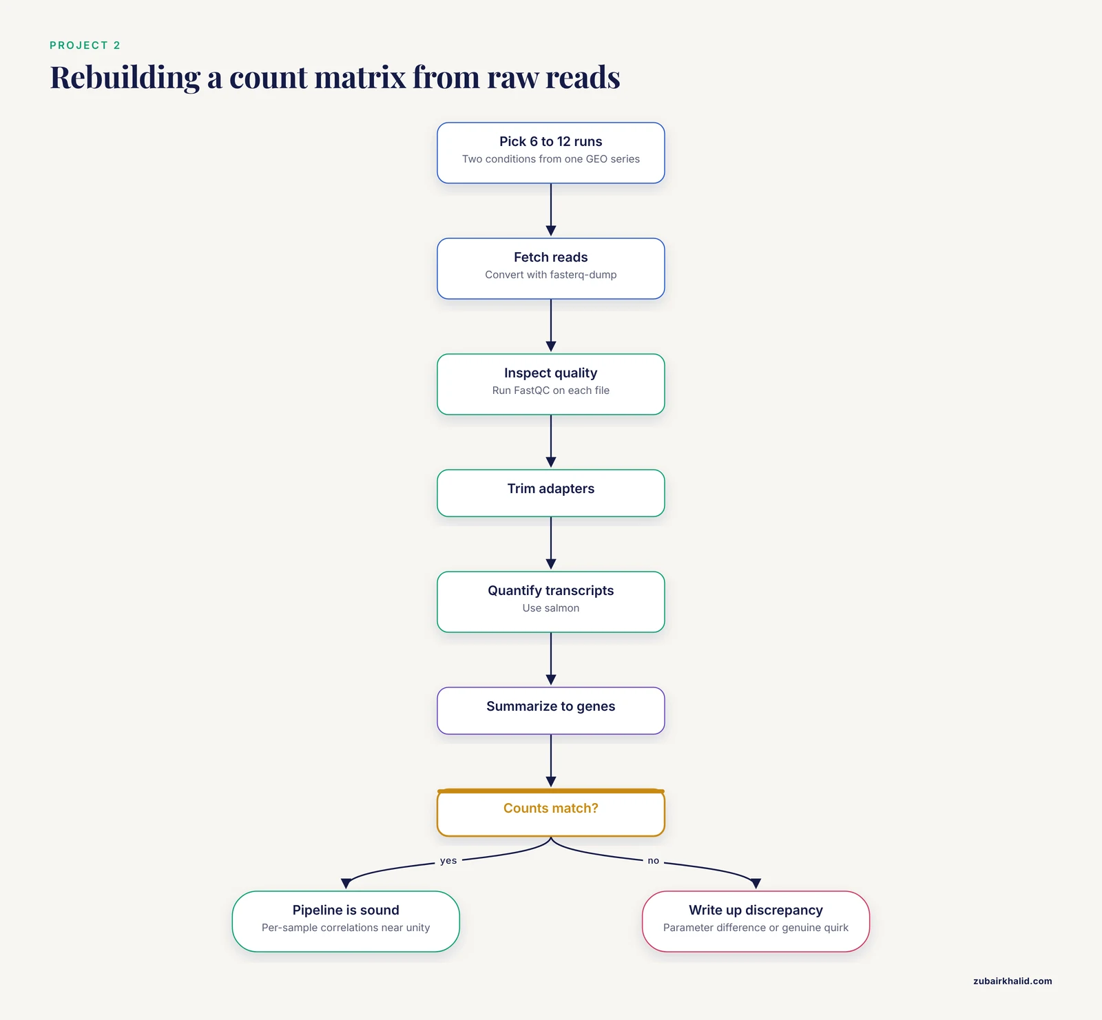
Branching workflow from SRA runs through fasterq-dump, FastQC, trimming and salmon to a count matrix compared against the deposited one.

Choose a modest GEO series with linked SRA runs and take 6 to 12 runs spanning two conditions. Fetch the reads with fasterq-dump, inspect them with FastQC, trim adapters, quantify transcripts with salmon, and summarize to gene-level counts. Compare your matrix to the deposited one, sample by sample. Finish line: per-sample correlations near unity and a written note on every discrepancy you found. This project teaches more per hour than anything else on this list because it touches every layer of the pipeline.

Project 3: A Team Reanalysis, Course Style

Mirror the Helsinki proteomics course [2]. Assign each team member one PRIDE project, agree on a shared R workflow (rpx to fetch, QFeatures to hold the assay, MSqRob2 or limma for statistics), and require everyone to record the parameters the original authors left undocumented. Compare reanalyzed results to the published ones and classify each discrepancy as metadata-driven, parameter-driven, or data-driven. Finish line: a short report per project plus one SDRF-formatted metadata sheet you authored yourself. As a bioinformatics course capstone or journal-club project, this format scales from two people to ten.

Project 4: Microbiome Diversity in One Afternoon

Load a packaged phyloseq object from a data-journal 16S dataset [11]. Compute alpha diversity per treatment group, run a Bray-Curtis ordination, and test whether community structure differs across the experimental systems. Finish line: figures that match the ones in the dataset's own HTML reports, produced by your code rather than theirs. When that feels easy, export the raw reads and rebuild the OTU table yourself with DADA2.

Project 5: Classify Genomes Without Aligning Them

Sample a few thousand genomes from a public viral collection, extract k-mer frequency vectors, and train a random forest to predict lineage, holding out entire lineages rather than random sequences [8]. Finish line: a confusion matrix you can defend, plus an honest paragraph on why lineage-level holdout yields lower apparent accuracy than random splitting. That paragraph is where the learning lives, because it forces you to define what "similar" means in your data.

Common Mistakes and Limitations

Treating processed files as analysis-ready. Deposited matrices arrive counts-normalized, log-transformed, or something in between, and the label is not always accurate. Check value ranges before modeling, and when in doubt, rebuild from raw counts.

Ignoring metadata until it hurts. The most common failure in public-data practice is downloading a matrix before reading the sample annotations. Without condition, batch, and pairing information, even a perfect matrix cannot answer a question. Absent metadata topped the recurring barriers found in the proteomics reanalysis study for good reason [2].

Assuming replication is automatic. Two studies reviewed here found the opposite: published classifiers lost accuracy on new cohorts [4], and student reanalyses diverged substantially from original proteomics results [2]. Expect divergence, diagnose it, and count the diagnosis as the win.

Downloading raw data without a compute plan. Raw proteomics files and large genome collections outgrow laptops quickly. Estimate storage and runtime before you download, and scale your first attempts down rather than up.

Overfitting your practice to one dataset. The RNA structure study showed training-data composition dominating predictor performance [9]. Rotate datasets. A finding that survives on two independent cohorts deserves more belief than one that appears once.

Skipping citation and license checks. Cite the accession and the companion paper wherever your work appears, and read the repository terms before redistributing files or results.

Mixing cohorts without harmonization. Combining TCGA tumors with GTEx normals, or pooling GEO series generated on different platforms, introduces systematic differences that can masquerade as biology. Model batch explicitly or restrict contrasts to within-program comparisons.

One boundary statement belongs here rather than anywhere else. Analyses of public datasets are for learning and research. They do not diagnose anyone, and individual clinical decisions belong with qualified clinicians who can order appropriate tests on real samples.

Frequently Asked Questions

What is the best starting point if I am completely new to bioinformatics?

Start with a packaged dataset from a data journal, because it arrives with metadata, processed objects, and a published analysis to compare against. Move to a GEO series with a count matrix once loading, plotting, and summarizing feel routine.

Where can I find raw sequencing reads to practice full pipelines?

The SRA holds raw reads, and most GEO series link directly to their SRA runs. Convert the reads to FASTQ, then work through quality control, trimming, and quantification until you can reproduce the deposited count matrix.

Do these datasets cost anything or require registration?

The repositories covered here are free to download. A few clinically sensitive datasets sit behind controlled access that asks for registration and a brief justification, so check the terms on the specific entry before planning a project around it.

How much computing power do I need?

Processed matrices and packaged R objects run comfortably on an ordinary laptop. Raw RNA-seq for a handful of samples is feasible locally or on a small cloud instance. Proteomics raw files and hundred-thousand-genome collections need more disk and memory than a laptop typically offers.

Can I publish an analysis I did on public data?

Yes. Reanalysis is an accepted research contribution, and several studies referenced in this guide are exactly that. Cite the accession and the original paper, follow the repository terms, and document your parameters well enough for someone to repeat your run.

How do I judge whether a dataset is good enough to practice on?

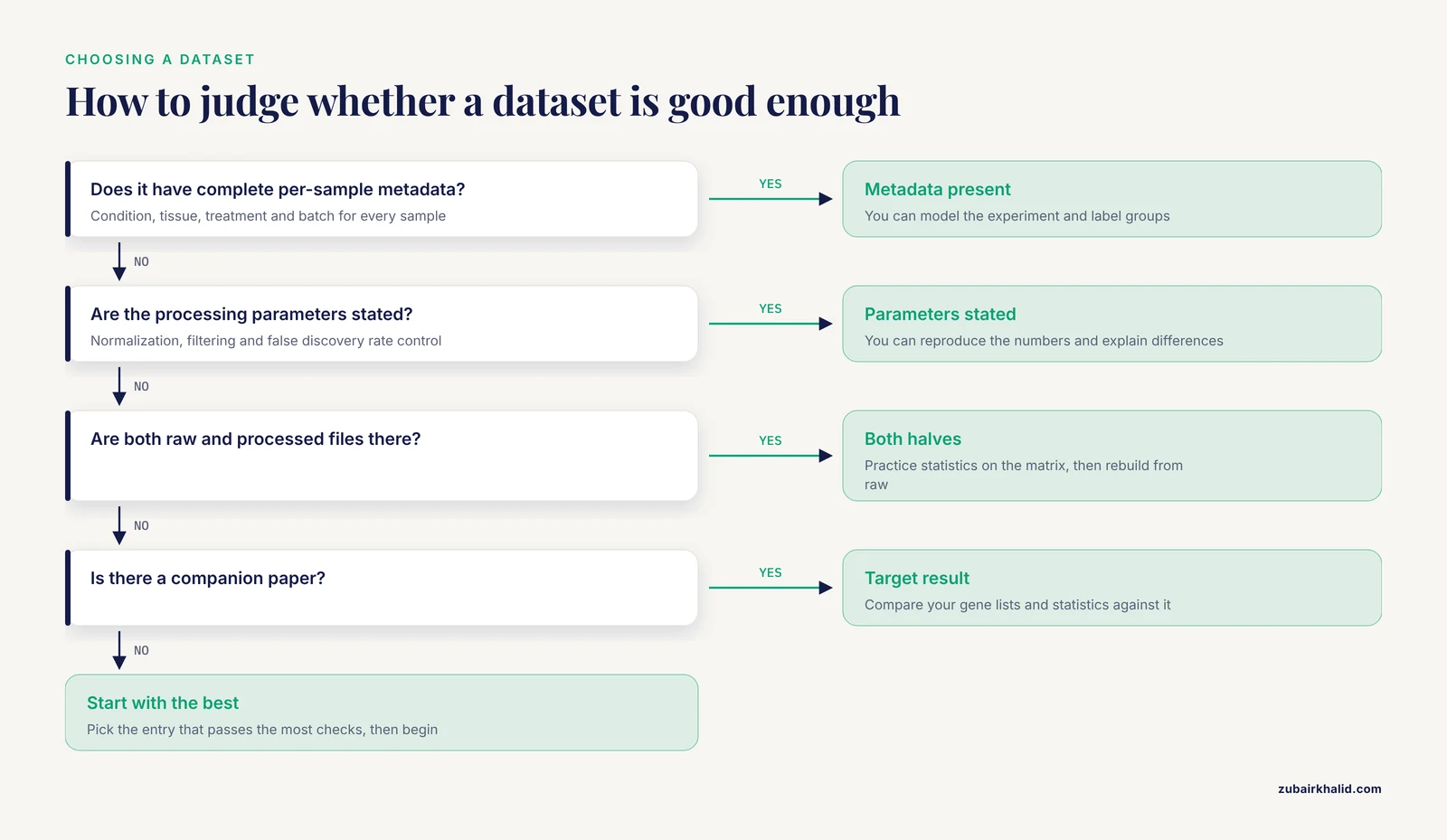
Decision path checking per-sample metadata, stated processing parameters, raw plus processed files and a companion paper before starting practice.

Look for four things: complete per-sample metadata, stated processing parameters, both raw and processed files, and a companion paper. A dataset missing most of those is still usable, but budget extra time for archaeology before any analysis.