How to Interpret Feature Importance in Genomic Models

By Dr. Zubair Khalid, DVM, MS, PhD · 2026-11-11

Feature importance in genomic models is the process of assigning a score to each gene, variant, CpG site, or genomic region that describes how much that feature contributed to a model's predictions. Interpreting those scores means translating a ranked list of features into a defensible biological or clinical claim, which requires checking the scores against statistical evidence, stability across data splits, and prior biological knowledge.

This topic matters because genomic models routinely drive decisions about biomarker discovery, patient subtyping, and drug resistance, and a model with excellent accuracy can still mislead you if its top features are artifacts. Recent evaluations of gene-level explanations show that different methods often disagree about which genes matter most, even when the models achieve similar accuracy, so interpretation is a distinct analytical step with its own quality controls rather than a byproduct of training [1].

What Feature Importance Means in Genomic Models

When people ask what feature importance interpretation in genomics with Python means, they are usually asking about a workflow with three parts. First, you train a supervised model, such as a random forest or a neural network, on a genomic feature matrix where rows are samples and columns are genes, variants, or regulatory regions. Second, you compute a per-feature score using a method such as impurity-based importance, permutation importance, SHAP values, or integrated gradients. Third, you interpret the top-scoring features biologically, which is the step where most errors happen.

The core problem is scale and correlation. A bulk RNA-seq matrix can contain 20,000 or more genes, a genome-wide SNP matrix can contain hundreds of thousands of variants, and a scChIP-seq dataset is sparse with mostly undetected regions [2]. Genes are correlated through co-regulation, variants are correlated through linkage disequilibrium, and the sample count is usually much smaller than the feature count. Under these conditions, a model can reach the same prediction using many different subsets of correlated features, and the importance score reflects which subset the algorithm happened to use, not necessarily the only biology involved.

A concrete example makes the stakes clear. In a study that trained machine learning models to classify cancer samples by type, a small set of top-ranked genes was sufficient to achieve good classification, but similar classification performance was achievable with lower-ranked genes when larger sets were used. Top-ranked genes differed substantially between statistical feature selection methods such as DESeq2 and learning-based attribution methods such as integrated gradients, which prevents a single comprehensive biological reading from any one ranking [1]. If you report only the top ten genes from one method, you are reporting one of several defensible stories.

The Main Families of Feature Importance Methods

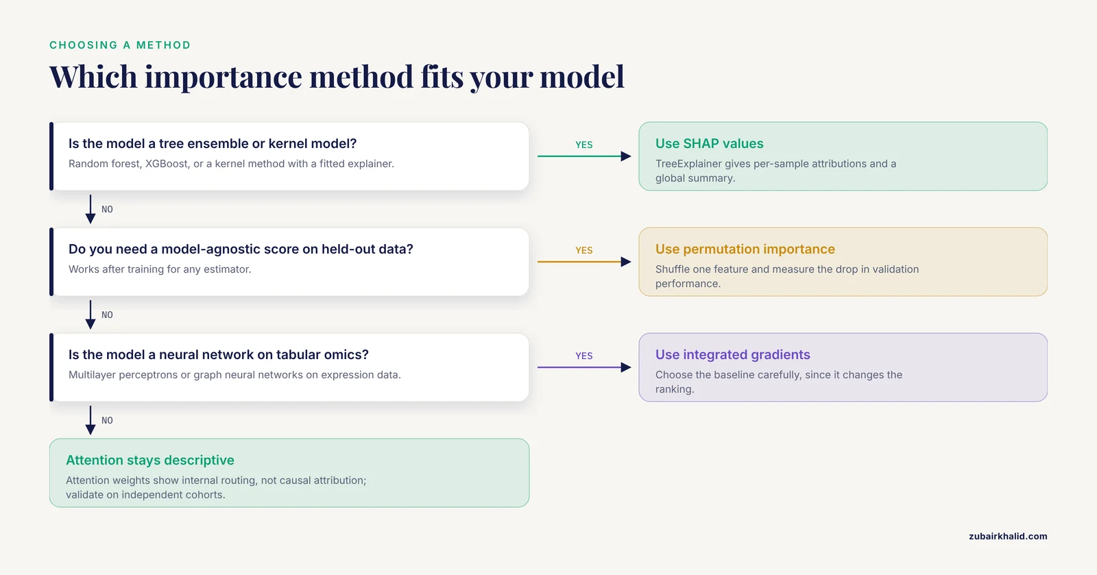
Decision path asking about model type and correlation, leading to permutation importance, SHAP, integrated gradients or attention weights.

Feature importance methods fall into four broad families, and knowing which family a score belongs to tells you what the score can and cannot support.

Intrinsic (model-native) importance. These scores come from the model structure itself. Random forest impurity importance sums the impurity reduction each feature provides across all splits, and coefficients in penalized logistic regression or elastic-net models act as importance weights. A study of antibiotic resistance prediction in Gram-negative pneumonia compared random forest, logistic regression, and XGBoost models built in Python 3.9.0 and screened predictive indicators through univariate and multivariate logistic regression before model construction [3]. The screening step matters because univariate association and model-based contribution are different questions, and features can score differently on each.

Perturbation-based importance. These scores measure how predictions change when you permute or perturb a feature. Permutation importance is the workhorse here because it is model-agnostic and works after training. Its weakness in genomics is correlation between features, since permuting one gene while its co-regulated partners stay intact can create biologically impossible inputs and underestimate the permuted gene's role.

Attribution methods for deep models. Integrated gradients attribute a prediction to input features by accumulating gradients along a path from a baseline input to the actual input. A comparative analysis used integrated gradients to rank genes in RNA-seq cancer classifiers built from multilayer perceptrons and graph neural networks, then compared those rankings against DESeq2 and other global contribution measures [1]. SHAP (Shapley Additive Explanations) values are the game-theoretic attribution standard for tree and kernel models, and they appear throughout applied genomics, from tissue-of-origin prediction to clinical subtyping audits [4], [5].

Structural and attention-based explanations. Attention weights in transformers and autoencoder bottlenecks provide a window into what the model focuses on internally, but attention is not a causal attribution and must be treated as descriptive. The ACSCeND framework for cancer stem-like cell classification uses an attention-guided autoencoder for bulk deconvolution, and its state-specific molecular programs come from combining attention structure with downstream validation across more than 25,000 tumor profiles from TCGA, PRECOG, and checkpoint inhibitor studies [6]. Similarly, SIMPA interprets per-cell imputation models for scChIP-seq by identifying the input genomic regions most important for each region-specific model, which turns an imputation pipeline into a source of single-cell regulatory hypotheses [2].

Quick reference table

Term	What the score measures	Typical tools	Most often confused with
Impurity importance	Training-time impurity reduction in tree splits	scikit-learn `feature_importances_`	True biological effect size
Permutation importance	Drop in validation performance when a feature is shuffled	`sklearn.inspection.permutation_importance`	Impurity importance, which uses no held-out data
SHAP value	Marginal contribution of a feature to an individual prediction, from Shapley values	`shap` package, TreeExplainer, KernelExplainer	Any generic importance score, and coefficient estimates [4], [5]
Integrated gradients	Path-integrated gradient attribution for neural networks	Captum, TensorFlow explainability APIs	Saliency maps from a single gradient evaluation [1]
Attention weight	Internal weighting of inputs within an attention layer	Model inspection in PyTorch	Causal or calibrated attribution [6]
Differential expression (DESeq2-style)	Statistical evidence that a feature differs between groups, independent of any model	DESeq2, edgeR, pyDESeq2	Feature importance, since a top model feature need not be the top DE gene [1]
Feature selection	Choosing a subset of features before or during training	Univariate filters, LASSO, mRMR	Importance ranking, since selection optimizes prediction, not explanation [1], [7]

A Reproducible Python Workflow, Step by Step

This section lays out the workflow you can adapt for gene expression, methylation, or SNP data. The commands use standard packages from the Python scientific stack, which is the core of Python for bioinformatics: pandas, scikit-learn, shap, and Biopython for annotation lookups.

Step 1: Prepare the feature matrix with the sample-to-feature orientation you will actually model

The most common setup is samples as rows and genes as columns. If your expression table is genes as rows, transpose it before training. Keep a separate held-out test set from the start, because importance computed on training data is not evidence of generalization.

import pandas as pd
from sklearn.model_selection import train_test_split

# expression.tsv: rows are genes, columns are samples
X = pd.read_csv("expression.tsv", sep="\t", index_col=0).T
y = pd.read_csv("labels.tsv", sep="\t", index_col=0)["cancer_type"]

X_train, X_test, y_train, y_test = train_test_split(
    X, y, test_size=0.25, stratify=y, random_state=42
)

Filter low-expression or low-variance features before modeling. In high-dimensional genomic data, feature filtering is not a threat to interpretation, it is a prerequisite, because noise features dilute every downstream ranking.

Step 2: Train a baseline model and record its honest performance

Use cross-validation on the training set before you look at any importance scores. A model whose performance is near chance produces importance scores that are noise with structure, and every hour spent interpreting them is wasted.

from sklearn.ensemble import RandomForestClassifier
from sklearn.model_selection import StratifiedKFold, cross_val_score

rf = RandomForestClassifier(n_estimators=1000, random_state=42)
cv = StratifiedKFold(n_splits=5, shuffle=True, random_state=42)
scores = cross_val_score(rf, X_train, y_train, cv=cv, scoring="roc_auc_ovr")
print(scores.mean(), scores.std())

The antibiotic resistance study cited above followed exactly this discipline, evaluating random forest, logistic regression, and XGBoost models with accuracy, precision, recall, F1 score, and the area under the receiver operating characteristic curve, then checking calibration curves and decision curves for clinical applicability before presenting biomarkers [3]. Calibration and decision-curve analysis are worth adopting whenever the model supports a clinical decision, because a well-ranked feature list from a miscalibrated model can still mislead practice.

Step 3: Compute three importance scores instead of one

Run impurity importance, permutation importance, and SHAP values side by side. Agreement between methods is weak evidence of robustness, and disagreement is diagnostic information.

from sklearn.inspection import permutation_importance

rf.fit(X_train, y_train)

# impurity-based, training-time only
impurity_imp = pd.Series(rf.feature_importances_, index=X.columns)

# permutation importance on held-out data
perm = permutation_importance(rf, X_test, y_test, n_repeats=30, random_state=42)
perm_imp = pd.Series(perm.importances_mean, index=X.columns)

# SHAP values for individual predictions
import shap
explainer = shap.TreeExplainer(rf)
shap_values = explainer.shap_values(X_test)

The SHAP step is where per-sample explanation becomes possible. MLMarker, a random forest tool for tissue-of-origin inference in proteomics, generates probabilistic predictions with SHAP-based protein-level explanations, with a penalty factor for missing proteins to stay robust on low-coverage samples [4]. That design point generalizes, in genomics your attribution method should account for missingness structure rather than silently imputing it, because an importance score for a feature the assay barely measured is not interpretable.

Step 4: Test the stability of the ranking across folds and resamples

A top feature that appears in one cross-validation fold but not the next is not a biomarker, it is a sample of the ranking variance. Re-fit the model within each training fold, collect the top-k features per fold, and summarize how often each feature appears. Report features that recur consistently, and report the churn rate itself, because a ranking that turns over almost completely between folds tells reviewers the dataset is underpowered for the claim being made.

The SNP-based schizophrenia prediction study illustrates the value of stratified structure in this process. The authors built ethnicity and sex specific models using stratified five-fold cross-validation, combined feature selection with association analysis to rank SNPs, and reported independent-test-set metrics for each group, with EA-F, EA-M, AA-F, and AA-M models reaching classification accuracies of 75.1 percent, 65.4 percent, 68.6 percent, and 73.9 percent respectively [7]. Stratifying by population before ranking features is itself an interpretation decision, because a variant important in one ancestry group can rank differently in another, and pooled rankings can hide that heterogeneity.

Step 5: Compare the model ranking against statistical evidence

Bring in the differential expression or association analysis as a second lens. For RNA-seq, run DESeq2 in R or pyDESeq2 in Python and overlay the two rankings. The comparative analysis of gene expression profiling showed significant differences in top-ranked genes between statistical selection and learning-based attribution, especially between DESeq2 and integrated gradients [1]. The practical rule is to treat features agreed on by both lenses as high-confidence candidates, and to investigate disagreement rather than average it away. A gene with strong differential expression that the model ignores may be redundant with a better-measured surrogate, and a gene the model ranks highly with no differential signal may be capturing a batch effect.

Step 6: Annotate features with Biopython before you write biological claims

Raw feature identifiers are not interpretation. Map Ensembl IDs or probe IDs to gene symbols and genomic coordinates, then pull functional context. A short Biopython example using the Entrez utilities to fetch gene records illustrates the pattern, and the same approach extends to batch annotation of hundreds of candidate genes.

from Bio import Entrez

Entrez.email = "you@your institution.org"
handle = Entrez.esearch(db="gene",
                        term="TP53[Gene Name] AND Homo sapiens[Organism]")
ids = Entrez.read(handle)["IdList"]
handle.close()

summary = Entrez.read(Entrez.esummary(db="gene", id=ids))
print(summary["DocumentSummarySet"]["DocumentSummary"]["Description"])

This annotation step is also where you check whether your top features are enriched for mitochondrially encoded genes, ribosomal genes, or known batch-correlated loci. Enrichment of those categories is a red flag that the ranking reflects technical structure rather than phenotype biology.

Step 7: Report the ranking with its uncertainty

For each reported feature, give the attribution value with its variability across repeats or folds, the direction of effect where the method supports one, and the per-sample SHAP distribution rather than only a global mean. A single-number ranking hides the skew and multimodality that often carry the biological story, for example a feature important in only one subclass of samples.

How Interpretation Is Tested in Practice

Interpretation is not finished when the ranking is computed. Mature workflows test interpretations against independent evidence in four ways.

Consistency checks across method families. Compute rankings with at least two method families and quantify rank agreement, for example with a Spearman correlation on the top 100 features. Large disagreement between statistical and learning-based rankings is a documented finding, not a failure of your code [1].

Performance-sufficiency probes. Ask how many top-ranked features are needed to recover most of the model's performance, and whether randomly selected lower-ranked features can do the same job. The integrated gradients analysis found that a small set of top-ranked genes sufficed for good classification, yet similar performance was achievable with larger sets of lower-ranked genes [1]. When lower-ranked features recover performance, the top of the ranking is a convenience, not a boundary of biological relevance.

External validation. Score the top features in an independent cohort or a different assay. MLMarker validated its SHAP-based tissue inference across three public datasets, finding brain-like signatures in cerebral melanoma metastases and identifying brain and pituitary origins in biofluids [4]. SyMetrics went further and validated predictions at the bench, performing functional assays on selected synonymous variants in the AVPR2 gene and using large-scale mutagenesis screens of RAD51C and BAP1 variants alongside its machine learning model, which achieved 97 percent accuracy with a ROC-AUC of 0.89 on genome-wide synonymous variant classification [8]. Functional validation of a handful of top features is the strongest interpretation evidence available, and the SyMetrics clinical follow-up, where 15 predicted deleterious variants appeared in genes linked to patient phenotypes with 9 classified as pathogenic or likely pathogenic and 6 as variants of uncertain significance, shows how a model ranking translates into a clinical review workflow [8].

Perturbation and counterfactual tests. For deep models, integrated gradients on a properly chosen baseline lets you attribute individual predictions to specific inputs, and SIMPA extended this logic to per-cell, per-region models in scChIP-seq, revealing which interaction sites drive each single-cell imputation [1], [2]. In sequence models, motif-level attribution can be validated by mutagenesis predictions, and DeepCC9 applied this idea to CRISPR-Cas9 guide design, combining explicit sequence feature extraction with a residual deep architecture and uncovering 74 sequence motifs enriched or depleted at specific sgRNA positions that were associated with editing efficiency [9]. When an attribution method points to positional sequence features that a wet-lab screen can verify, the interpretation loop closes.

Interpreting Importance in Deep Genomic Models

Deep models dominate modern genomics, from graph neural networks on gene interaction networks to CNNs on sequence data, and their importance interpretation has its own vocabulary and pitfalls.

Integrated gradients is the reference attribution method for neural networks on tabular omics data. It satisfies axioms that practitioners care about, including sensitivity, meaning features that differ between input and baseline receive nonzero attribution, and completeness, meaning attributions sum to the difference between the prediction and the baseline prediction. In practice you choose a baseline carefully, often a zero vector or a per-feature median, because the baseline changes the ranking, and the cancer classification study made baseline-dependent disagreement between attribution methods and statistical selection a central finding [1].

For attention-based architectures, the honest position is that attention weights describe internal information routing. ACSCeND uses an attention-guided autoencoder for deconvolving cancer stem-like cell subtype proportions from bulk RNA-seq, and the framework's biological claims rest on correlations validated across more than 25,000 tumor profiles, including the finding that CSC abundance correlates with poor disease-free survival and reduced immunotherapy efficacy [6]. The attention mechanism organizes the representation, the cohort-level validation carries the claim. Conflating the two is a common error in papers and reviews.

For sequence models, position-resolved attribution is often the most biologically productive output. DeepCC9's analysis of composition and position based motifs demonstrates the payoff, since its 74 position-specific motifs provide mechanistic hypotheses about Cas9 guide performance that simpler black-box predictors could not offer [9]. The transferable lesson is to design the architecture and the attribution granularity together, so that the explanation matches a unit of biology, a motif, a CpG, a chromatin region, rather than an arbitrary pixel of the input.

Python Tooling Beyond the Core Stack

A few packages deserve specific mention because they shape how interpretation is done in genomics workflows.

pyVIPER brings protein activity inference and master regulator analysis to single-cell RNA-seq in Python, with a data structure for manipulating gene regulatory networks, integration with scverse and scanpy, and PyTorch-based GPU acceleration that reduces analysis time for large datasets from hours to minutes compared with the R implementation [10]. Master regulator analysis is itself a form of importance interpretation, moving the unit of explanation from individual genes to regulatory proteins, which often aligns better with mechanism.

ultra-impute addresses the input problem, since a two-stage framework for systematic missing values in DNA methylation arrays uses multi-output models including support vector regression, random forest, and deep neural networks, and imputing missing CpG sites improved epigenetic age prediction performance [11]. The connection to interpretation is direct, missingness handling changes which features appear complete enough to trust, so imputation choices propagate into importance rankings.

mmContext shows where the field is heading, learning joint embeddings of omics data and text with contrastive objectives so that cell types and diseases can be classified zero-shot across independent datasets, with pretrained checkpoints released openly [12]. In such models, importance interpretation may shift from individual features to embedding dimensions and retrieved text anchors, and the evaluation discipline, held-out datasets and released artifacts, is the part worth copying now.

Agentomics represents the automation layer, an agentic system that implements machine learning strategies end to end with strict validation checkpoints and outperformed other agentic systems across 20 datasets spanning protein engineering, drug discovery, and regulatory genomics [13]. For interpretation, the relevant point is the checkpoint design. Automated pipelines that lock in validated artifacts before moving steps make it harder for an importance analysis to run against an incorrectly split or leaked dataset, which is one of the most common silent failures in applied genomic machine learning.

Terms Feature Importance Is Confused With

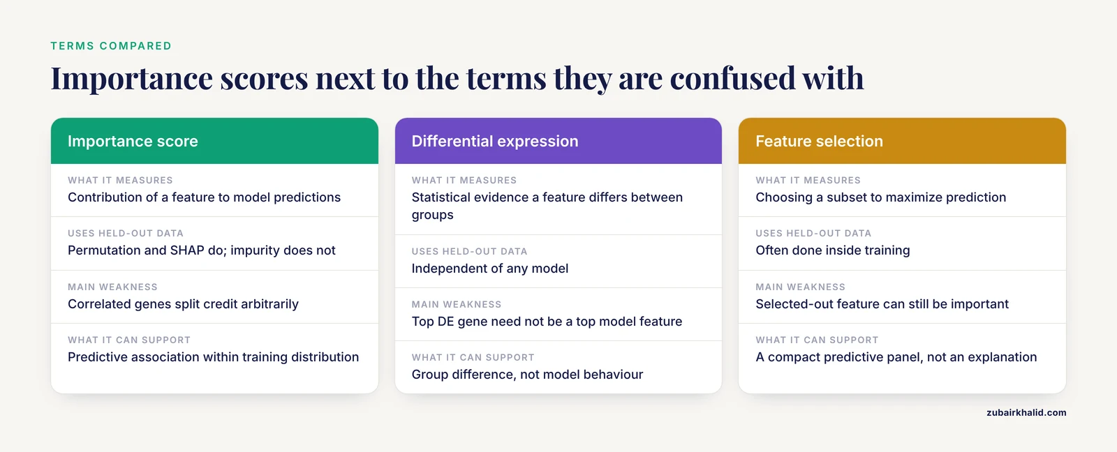
Comparison of importance scores with differential expression and feature selection on what each measures, held-out data use, weakness and support.

Students most often blur four pairs of concepts.

First, feature importance versus feature selection. Selection chooses a subset to maximize prediction, importance scores contributions to explain predictions, and a selected-out feature can still be biologically important if a correlated proxy was selected instead [1].

Second, importance versus differential expression. A gene can be the strongest DESeq2 hit and irrelevant to a classifier that uses other correlated genes, and conversely a top model gene can carry modest differential signal [1]. Report both analyses and their overlap.

Third, global importance versus local explanation. A global ranking summarizes contributions across the dataset, while a SHAP value or integrated gradient attribution explains one prediction. MLMarker provides both levels, population-level tissue similarity scores and protein-level SHAP explanations per sample [4], and reporting only the global level hides subclass-specific mechanisms.

Fourth, association versus mechanism. A high importance score is evidence of predictive association within the training distribution. The SyMetrics workflow shows what moving toward mechanism requires, functional assays and segregation data layered on top of the model output [8].

Quick Review

Feature importance scores rank genomic features by their contribution to model predictions, and interpreting them is a separate, error-prone analytical step [1].
Use at least two importance method families, such as permutation importance and SHAP, and treat disagreement as information [1],.
Compute importance only after honest cross-validated performance is established, and always on held-out data for perturbation methods [3].
Test ranking stability across folds and ancestry or subclass strata before naming biomarkers.
Overlay model rankings with statistical analyses such as DESeq2, and investigate overlap and disagreement explicitly [1].
Validate top features externally, in independent cohorts when possible, and functionally when the stakes justify it, [8].
For deep models, match attribution granularity to a unit of biology such as a motif or regulatory region, and never present attention weights as causal evidence [6], [9].

Common Mistakes and Limitations

Trusting impurity importance on high-cardinality or correlated features. Impurity importance is biased toward continuous and high-cardinality features and splits credit arbitrarily among correlated genes. Use it as a quick look, never as the reported result.

Interpreting importance from a leaking pipeline. If normalization parameters, feature filtering, or imputation were fit on the full dataset before splitting, both performance and importance are contaminated. Fit every preprocessing step inside the cross-validation loop. This is the class of error that validation checkpoints in automated systems are designed to catch [13].

Ignoring missingness. Genomic assays have structured missingness, from low-coverage proteomics to sparse scChIP-seq. A feature with near-zero detection in your cohort can receive high apparent importance purely from imputation artifacts, which is why methods that explicitly penalize missing proteins, as MLMarker does, report more trustworthy attributions [4], [2].

Reading the top of the ranking as the whole story. The documented result that similar classification performance is achievable with lower-ranked genes means the top-k cutoff is a presentation choice [1]. Report how quickly performance recovers as you add features, and state the cutoff you chose.

Assuming a single true ranking exists. Different valid methods produce different rankings on the same data [1]. The goal of interpretation is a robust set of candidate features supported by multiple lenses, not the one canonical list.

Confusing local with global explanation. A mean SHAP value across samples can average away a mechanism present in one subtype. Inspect per-sample attributions, especially in heterogeneous tumors.

Skipping batch and ancestry checks. If your top features separate samples by sequencing batch, processing date, or population structure, the ranking describes those variables. Always regress or visualize top features against known technical and demographic covariates before biological interpretation [7].

Treating clinical deployment as a solved problem once importance looks plausible. The antibiotic resistance workflow paired its model metrics with calibration curves and decision curves, because feature plausibility does not establish clinical utility [3]. Individual predictions from any genomic model require review by a domain expert before they inform patient care.

Finally, remember the boundary of the evidence itself. Attribution methods explain the model, and only secondarily the biology. When the model is mis-specified, trained on biased sampling, or underpowered, a beautifully stable importance ranking is a stable description of the wrong thing.

Frequently Asked Questions

What does feature importance interpretation in genomics with Python mean?

It means training a supervised model on genomic features such as genes, variants, or CpG sites, computing a per-feature contribution score with tools like scikit-learn or SHAP, and then validating that ranking against statistical analyses, stability checks, and biological knowledge. Interpretation is the validation and translation step, not the score computation itself.

Which feature importance method should I use for gene expression data?

Use at least two. Permutation importance on held-out data and SHAP values from a tree ensemble are a practical pair for expression matrices, and you should overlay the results with DESeq2-style differential expression because statistical and learning-based rankings are known to disagree substantially on top genes [1]. Agreement between methods is your minimum robustness bar.

Why do my top-ranked genes change between cross-validation folds?

Rankings are estimates with variance, and in high-dimensional, correlated, small-sample genomic data that variance is large. Genes correlated with a true signal gene can swap places across folds without changing model performance. Report how often each feature recurs across folds and treat single-fold top genes as unstable [1].

Can SHAP values tell me which genes cause the disease?

No. SHAP values explain what a specific model used to make a specific prediction, which is association within your training distribution, not causation. Causal claims require interventions, such as the functional assays and mutagenesis screens used to validate variant predictions in SyMetrics [8], or perturbation experiments outside the model.

How do I interpret feature importance in a neural network trained on genomic data?

Use gradient-based attribution such as integrated gradients, which was evaluated on RNA-seq cancer classifiers and compared against statistical selection methods, and be explicit about your baseline choice since it affects the ranking [1]. For sequence models, extract position-resolved motifs so the attribution maps to a biological unit, following the motif and position analysis approach of interpretable CRISPR guide models [9]. For attention architectures, treat attention as descriptive and validate the derived biology on independent cohorts [6].

How many top features should I report from a genomic model?

Report the number that the performance analysis supports, not a fixed number. Because good classification can be achieved with a small top set and similar performance is possible with larger sets of lower-ranked genes, present the performance-versus-feature-count curve and justify your cutoff [1]. For sparse single-cell settings, very small feature sets can carry substantial signal, as imputation models for scChIP-seq were trained with only 100 input genomic regions to predict thousands of undetected regions [2].