Clustering Gene Expression Data with scikit-learn
By Dr. Zubair Khalid, DVM, MS, PhD ·

KMeans assigns every sample to exactly one of a fixed number of round-shaped groups you choose in advance, while DBSCAN finds groups of any shape from dense neighborhoods and leaves outliers unlabeled, so the right starting choice depends on whether you know how many groups you expect and whether your samples contain true outliers. The practical rule of thumb: use KMeans when you have a good guess for the number of groups and your data are roughly spherical after PCA, use hierarchical clustering when you want a dendrogram and have fewer than about 20,000 samples, use DBSCAN when cluster shapes are irregular or outliers matter, use Gaussian mixture models when cluster membership is genuinely fuzzy, and use graph-based clustering when you are working with single-cell data at scale.
This guide walks through the full workflow for clustering gene expression data with scikit-learn, compares the main algorithm options with their pros and cons, gives worked code you can adapt, and covers the preprocessing and evaluation steps that decide whether your clusters mean anything biologically.
Why Python and scikit-learn for gene expression clustering
Python has become the default scripting language for bioinformatics work that goes beyond sequence file handling. Interactive Jupyter notebooks are now widely used to teach computational analysis in the life sciences, with cloud-based frameworks delivering preconfigured Python environments and version-controlled notebooks so that analyses run consistently across different machines [1]. That reproducibility matters in clustering work specifically, because small changes in preprocessing can move samples between clusters.
scikit-learn sits at the center of this ecosystem for three reasons:
- Every algorithm follows the same
fitandpredictinterface, so swapping KMeans for a Gaussian mixture model is a one-line change. - It ships with the preprocessing tools (scaling, PCA, sparse-matrix handling) and the validation metrics (silhouette, adjusted Rand index) that clustering pipelines need.
- It composes cleanly with the rest of the scientific Python stack, which is exactly how published transcriptomic analyses use it. A cross-cancer transcriptomic study, for example, performed unsupervised clustering of expression module scores in Python using scipy, scikit-learn, networkx, and matplotlib together [2].
A quick note on where Biopython fits. If you are following a Biopython tutorial for the first time, you will find that Biopython handles sequence objects, retrieval from NCBI Entrez, and annotation parsing. It is not a clustering library, and most gene expression analyses do not pass through Biopython at all. Expression data usually arrive as a count matrix or a microarray intensity table, which you load with pandas or the scanpy AnnData format. Biopython is useful upstream, for example to fetch gene annotations or sequences that you then map onto your expression matrix. Keeping the two roles separate prevents a common beginner confusion: clustering gene expression data with scikit-learn happens on numeric matrices, and Biopython handles the sequence side of the project.
The core workflow
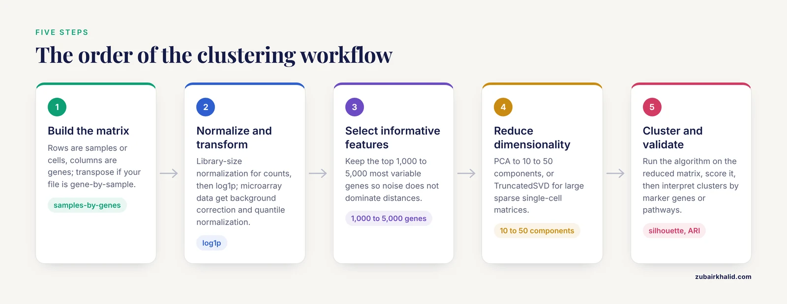
Every clustering analysis for expression data follows the same five steps. Getting the order right matters more than the choice of algorithm.
Step 1: Represent the data as a samples-by-genes matrix
Clustering can be applied in two directions. Cluster the rows (samples, patients, cells) to find subgroups with similar expression profiles, or cluster the columns (genes) to find co-expressed modules. Most workflows do both at different stages. The matrix is typically:
- Raw counts for RNA-seq (integer counts per gene per sample)
- Normalized intensities for microarrays
- Cell-by-gene counts for single-cell RNA-seq, stored sparse because most entries are zero
import pandas as pd

# rows = samples, columns = genes
expr = pd.read_csv("counts.csv", index_col=0)
X = expr.T          # transpose so rows are samples if your file is gene-by-sample
Step 2: Normalize and transform
Raw counts are not comparable across samples because of differences in sequencing depth. Standard practice for bulk RNA-seq is library-size normalization (counts per million, or a median-of-ratios method) followed by a log transform, usually log1p, which stabilizes variance so that a few highly expressed genes do not dominate every distance calculation. For microarray data, background correction and quantile normalization are the conventional steps.
For single-cell data, the scanpy ecosystem is the standard companion to scikit-learn. pyVIPER, a Python package for protein activity estimation from single-cell RNA-seq, was designed to integrate with scverse, scanpy, and widely adopted machine learning libraries, which reflects how deeply these tools are now interlinked [3].
Step 3: Select informative features
With tens of thousands of genes, distance calculations are dominated by noise. The standard fix is to keep the most variable genes, typically the top 1,000 to 5,000 by normalized dispersion, before clustering. This is standard textbook practice rather than a hard rule, and the right number depends on the biological signal you expect.
Missing values are a separate problem. Calling KMeans on a matrix with NaN values fails immediately. Simple options include dropping genes with missing values in more than a fixed fraction of samples, or median imputation. For systematically missing data, learned imputation models outperform simple filling, and one recent framework for DNA methylation arrays used support vector regression, nearest-neighbor methods, random forest models, and deep neural networks for this purpose, implemented in a Python package built on scikit-learn-style tooling [4]. Those ideas transfer directly to expression matrices with structured missingness.
Step 4: Reduce dimensionality
PCA is the near-universal intermediate step between preprocessing and clustering. It compresses correlated genes into a small number of orthogonal components, typically 10 to 50, which both denoises the data and makes distance-based clustering faster and more stable.
from sklearn.preprocessing import StandardScaler
from sklearn.decomposition import PCA

Xs = StandardScaler().fit_transform(X)
Xpca = PCA(n_components=20, random_state=0).fit_transform(Xs)
For large sparse single-cell matrices, use TruncatedSVD instead of dense PCA, since it operates on sparse input without densifying the matrix.
The number of components is a tuning decision. A common heuristic is to keep components until the explained variance curve flattens, or to retain 10 to 50 components for single-cell data and inspect the elbow plot. Clustering on too few components merges real subpopulations, and clustering on too many lets noise drive the distances.
Step 5: Cluster and validate
Only now do you apply a clustering algorithm. Every algorithm below takes this reduced matrix as input. After clustering, you validate with internal metrics or external metrics if you have reference labels, then interpret the clusters by checking marker genes or enriched pathways. A cluster with no interpretable biology is usually an artifact of your parameters, not a discovery.
Clustering gene expression python scikit-learn options: the comparison table
The table below is the core reference for the rest of the article. All of these classes exist in scikit-learn and accept the PCA-reduced matrix from the workflow above.
| Algorithm | scikit-learn class | Need k in advance? | Handles non-convex shapes? | Scales to | Assigns outliers to a cluster? | Best use case | Main drawback |
|---|---|---|---|---|---|---|---|
| KMeans | KMeans, MiniBatchKMeans | Yes | No | Millions of rows | Yes, always | Bulk samples with expected spherical groups | Forced equal-ish cluster sizes, wrong for elongated clusters |
| Bisecting KMeans | BisectingKMeans | Yes | No | Millions of rows | Yes, always | Large datasets with a hierarchical flavor | Still assumes variance-based splitting |
| Agglomerative hierarchical | AgglomerativeClustering | Optional (distance_threshold) | Partly, with average/complete linkage | About 20,000 samples before memory becomes the limit | Yes, always | Small cohorts where a dendrogram is wanted | Quadratic memory cost, irreversible merges |
| DBSCAN | DBSCAN | No (has eps, min_samples instead) | Yes | Tens of thousands | No, marks noise | Irregular cluster shapes, outlier detection | Sensitive to eps, struggles with varying density |
| Gaussian mixture | GaussianMixture, BayesianGaussianMixture | Yes | Elliptical only | Tens of thousands | Soft probabilities | Overlapping, ellipsoidal subpopulations | Numerical problems in very high dimensions, needs regularization |
| Spectral | SpectralClustering | Yes | Yes | Thousands to low tens of thousands | Yes, always | Non-convex structure on moderate-sized data | Costly eigendecomposition, needs affinity choice |
| kNN graph + community detection | NearestNeighbors (then Leiden/Louvain outside sklearn) | Resolution parameter, not exact k | Yes | Hundreds of thousands of cells | Depends on method | Single-cell RNA-seq at scale | The graph step is outside scikit-learn, more moving parts |
The algorithms on their own terms
KMeans
KMeans minimizes the within-cluster sum of squared distances to cluster centers. It is the default first attempt for clustering gene expression data with scikit-learn because it is fast, deterministic enough with a fixed random_state, and trivially interpretable.
from sklearn.cluster import KMeans

km = KMeans(n_clusters=4, n_init=10, random_state=0)
labels = km.fit_predict(Xpca)
Pros:
- Fastest general-purpose option, with
MiniBatchKMeansavailable for datasets that exceed memory. - Cluster centers can be inspected directly, and the distance of each sample to its assigned center is a useful confidence signal.
- Behaves predictably, which makes parameter sweeps straightforward.
Cons:
- You must fix
n_clustersin advance. - It implicitly assumes clusters are convex and roughly similar in size and variance. Elongated or crescent-shaped structures get split or merged incorrectly.
- Every sample is assigned, including samples that belong to no real group. Outliers become their own spurious cluster or get dragged into an existing one.
- Results depend on initialization, so run with
n_init=10or higher.
Bisecting KMeans
BisectingKMeans builds clusters hierarchically by repeatedly splitting the cluster with the largest variance. It produces a tree structure you can cut at different depths, often at lower computational cost than full agglomerative clustering. It shares KMeans' spherical assumption, so the same caveats about cluster shape apply.
Agglomerative hierarchical clustering
AgglomerativeClustering starts with every sample as its own cluster and iteratively merges the closest pairs. With n_clusters=None and a distance_threshold, you get a data-driven number of clusters instead of a fixed one. Ward linkage, which minimizes within-cluster variance, is the standard choice for expression data, and it pairs naturally with Euclidean distances on scaled, PCA-reduced matrices.
from sklearn.cluster import AgglomerativeClustering

agg = AgglomerativeClustering(n_clusters=None, distance_threshold=25, linkage="ward")
labels = agg.fit_predict(Xpca)
For the dendrogram itself you need scipy's linkage and dendrogram functions, since scikit-learn does not plot trees. This is one of the small friction points in an otherwise uniform API.
Pros:
- The dendrogram shows structure at every resolution at once, which is genuinely useful when you do not know whether your data contain 3 or 30 groups.
- No need to commit to k if you use a distance threshold.
- Ward linkage behaves well on standardized expression data.
Cons:
- Memory scales quadratically, so it becomes impractical for large single-cell datasets. Compute a condensed distance matrix and plan for roughly 20,000 samples as a practical ceiling on typical hardware.
- Merges are irreversible. A bad early merge propagates all the way up the tree.
- No
predictmethod for new samples. Assigning a new patient or cell requires nearest-centroid logic you write yourself.
DBSCAN
DBSCAN defines clusters as dense regions separated by sparse regions. Two parameters control it: eps, the neighborhood radius, and min_samples, the minimum points required to form a dense region. Points in low-density areas are labeled -1, meaning noise, and that behavior alone makes DBSCAN valuable for quality control in expression datasets with dead cells or failed samples.
from sklearn.cluster import DBSCAN
from sklearn.neighbors import NearestNeighbors
import numpy as np

# a data-driven eps: distance to the k-th nearest neighbor
nn = NearestNeighbors(n_neighbors=10).fit(Xpca)
dists, _ = nn.kneighbors(Xpca)
eps = np.percentile(dists[:, -1], 90)

db = DBSCAN(eps=eps, min_samples=10)
labels = db.fit_predict(Xpca)
Pros:
- No preset cluster count. The data determine how many groups exist.
- Outliers are identified explicitly instead of being forced into a cluster.
- Finds arbitrarily shaped clusters.
Cons:
- Performance is highly sensitive to
eps. A knee plot of sorted k-nearest-neighbor distances is the standard diagnostic for choosing it. - Clusters of varying density cause trouble, because a single global
epscannot serve both dense and sparse regions well. - In high dimensions, distances concentrate and density estimates become unreliable, which is why you cluster on PCA components rather than raw genes.
Gaussian mixture models
GaussianMixture fits a weighted sum of multivariate Gaussian distributions using expectation-maximization. Unlike KMeans, it returns soft assignments, the posterior probability that each sample belongs to each cluster, and it allows ellipsoidal clusters with per-cluster covariance.
from sklearn.mixture import GaussianMixture

gmm = GaussianMixture(n_components=4, covariance_type="full",
                      reg_covar=1e-5, random_state=0)
probs = gmm.fit_predict_proba(Xpca) if hasattr(gmm, "fit_predict_proba") else gmm.fit(Xpca)
labels = gmm.predict(Xpca)
probs = gmm.predict_proba(Xpca)
Setting reg_covar to a small positive value prevents the degenerate covariance errors that appear when a cluster collapses onto a few nearly identical samples, a frequent problem with gene expression inputs.
Pros:
- Soft membership captures genuine biological ambiguity, such as cells caught mid-transition between states.
BayesianGaussianMixturewith a highn_componentsprunes unused components automatically, which gives you a data-driven estimate of cluster number.- Ellipsoidal clusters fit more real expression data than KMeans' spherical assumption.
Cons:
- Slowest of the standard options on large data.
- Sensitive to initialization. Run with several
n_initvalues and compare. - Struggles in high dimensions unless you reduce first, and it requires more careful regularization than KMeans.
Spectral clustering
SpectralClustering builds an affinity graph between samples, computes the graph Laplacian's eigenvectors, and clusters in that embedding space. It excels at connected, non-convex structures that break KMeans, and it is the conceptual bridge between distance-based clustering and the graph-based methods that dominate single-cell analysis.
Pros:
- Handles intertwined or ring-shaped cluster structure.
- The affinity matrix can encode domain knowledge, for example a precomputed kNN graph.
Cons:
- Requires k in advance.
- The eigendecomposition makes it expensive on large datasets.
- Results depend heavily on the affinity construction, adding a layer of tuning on top of k.
Graph-based clustering for single-cell data
Single-cell RNA-seq changed the default clustering strategy. At hundreds of thousands of cells, pairwise-distance methods become infeasible, so the standard workflow builds a shared nearest-neighbor graph and applies graph community detection. A recent lightweight tool, SUMA, addresses a specific weakness of this approach: results depend strongly on the number of neighbors used to build the graph, so SUMA uses a random forest model built and optimized with scikit-learn to predict the optimum number of neighbors for a given dataset, with clustering quality assessed by adjusted Rand index against known labels [5].
Within scikit-learn itself, you can build the neighbor graph with NearestNeighbors or kneighbors_graph and then either cluster it with SpectralClustering or export it to igraph or leidenalg for Louvain and Leiden clustering. The scverse ecosystem wraps this whole pipeline, but the scikit-learn components underneath are the same ones described above.
The preprocessing lesson from the single-cell literature generalizes. CIRCE, a scalable Python package for predicting cis-regulatory interactions, benchmarked preprocessing choices and observed that Cicero's count normalization had a negative impact while working directly from the single-cell count matrix gave the best performance, and it introduced metacells, grouping of similar cells, to reduce sparsity [6]. The transferable insight is that normalization choices are empirical decisions to be tested, not defaults to be trusted, and that aggregating similar units can rescue sparse data before clustering.
Choosing the best clustering approach for gene expression data
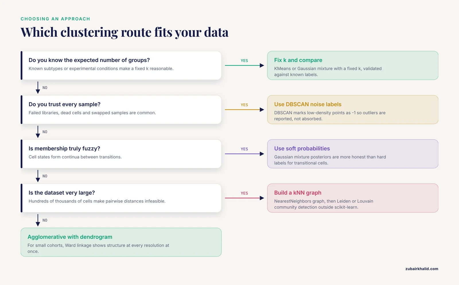
The "best clustering gene expression python scikit-learn" question has no single answer, but it does have a decision procedure. Work through these criteria in order.
Do you know the expected number of groups?
If you have prior knowledge, for example known subtypes or experimental conditions, external validation against those labels is possible, and KMeans or GMM with a fixed k is reasonable. If k is unknown, run the algorithm across a range of k and compare internal metrics, or use DBSCAN or BayesianGaussianMixture to let the data propose the count. Automated ML systems formalize this search, and Agentomics, an agentic system for biomedical machine learning, introduces strict validation checkpoints at standard development steps so that each modeling decision is validated before the next builds on it [7]. Even without such tooling, the same discipline applies to clustering: fix a preprocessing version, sweep parameters, and record every result.
Do you trust every sample?
Expression matrices routinely contain failed libraries, dead cells, or swapped samples. If outlier identification matters, DBSCAN's explicit noise label is a significant advantage. With KMeans, outliers contaminate cluster centers silently.
Is membership truly fuzzy?
Cell states form continua. If your question involves transitional populations, GMM probabilities are more honest than hard labels. If your question requires discrete groups, for example assigning samples to subtypes for downstream tests, hard clustering is appropriate and you should report assignment confidence separately.
How large is the dataset?
For up to a few thousand samples, all options are on the table and hierarchical clustering with a dendrogram is informative. For tens of thousands, KMeans, DBSCAN, and GMM remain practical. For hundreds of thousands of cells, use the kNN graph route, and consider metacell-style aggregation as CIRCE demonstrated, processing a dataset of more than 700,000 cells and 1 million DNA regions in under an hour with that strategy [6].
Evaluation metrics that actually decide the choice
Internal metrics require no ground truth:
silhouette_score: ranges from -1 to 1, higher is better, and values near zero indicate overlapping clusters. Computed on the same matrix you clustered on.calinski_harabasz_scoreanddavies_bouldin_score: fast alternatives for parameter sweeps, with higher and lower being better respectively.
External metrics require reference labels:
adjusted_rand_score(ARI): the standard reported measure in the clustering literature. An ARI of 1 is perfect agreement and 0 is chance level. SUMA used ARI against true cell labels to assess clustering quality across a wide range of neighbor and gene settings [5], and AESTETIK reported a 21% increase in median ARI over previous state-of-the-art methods on structured tissues such as brain in spatial transcriptomics [8].
from sklearn.metrics import silhouette_score, adjusted_rand_score

sil = silhouette_score(Xpca, labels)
ari = adjusted_rand_score(true_labels, labels)
A practical sweep looks like this:
import numpy as np
from sklearn.cluster import KMeans
from sklearn.metrics import silhouette_score

for k in range(2, 11):
    lab = KMeans(n_clusters=k, n_init=10, random_state=0).fit_predict(Xpca)
    print(k, silhouette_score(Xpca, lab))
Interpret the silhouette curve with the biology in mind. A flat curve across many k values usually means the data lack clean structure at that resolution, not that any k is fine.
Worked scenarios
Scenario 1: A bulk RNA-seq cohort of 200 patients
You have tumor and normal samples, and you suspect molecular subtypes within the tumors. Load the count matrix, normalize for library size, apply log1p, keep the top 2,000 most variable genes, scale, reduce to 20 PCA components, and run KMeans for k from 2 to 8 while tracking silhouette scores. Then run the winning k a second time with different random_state values to confirm stability. Follow up by testing whether clusters differ in survival or response, and report cluster-specific marker genes. If a handful of samples sit far from every center, rerun with DBSCAN on the same PCA space and check whether the same samples come out as noise, which is a useful robustness check.
This pattern mirrors published practice. In the cross-cancer transcriptomic analysis cited earlier, the authors computed module scores as mean z-scores across curated gene sets and applied unsupervised clustering in Python, using scikit-learn alongside scipy, networkx, and matplotlib to characterize conserved transcriptional programs [2]. Reducing genes to a small number of biological modules before clustering is a strong noise-reduction strategy worth borrowing for any cohort analysis.
Scenario 2: A single-cell dataset of 50,000 cells
Cluster on the kNN graph route. Normalize counts, log transform, identify highly variable genes, scale and reduce with PCA, build a neighbor graph with NearestNeighbors, and cluster with Leiden or Louvain at several resolutions. Because the neighbor count materially changes results, and because a model can predict a good value for it rather than guessing [5], treat n_neighbors as a tuned parameter and record it alongside the resolution. For downstream interpretation, pyVIPER-style protein activity analysis integrates directly with the scanpy objects you already have, giving a mechanistic layer on top of the clusters [3].
If your clusters look like a single merged blob, the usual culprits are too few PCA components, uncorrected batch effects, or overly aggressive normalization. If they fragment into dozens of tiny groups, increase min_samples in a DBSCAN check, raise the Leiden resolution threshold, or reconsider your highly variable gene selection.
Scenario 3: Spatial transcriptomics
Spatial platforms add tissue geometry to the expression matrix. Purely expression-based clustering ignores morphology, and modern methods learn joint representations of spatial context, transcriptomics, and image features before clustering. AESTETIK, a convolutional deep learning model for spatially resolved transcriptomics, improved cluster assignments across 10x Genomics and NanoString platforms, with gains of 2-fold in breast cancer, 79% in melanoma, and 21% in liver cancer samples relative to previous methods [8]. For a scikit-learn-centric workflow, the practical adaptation is to append spatial coordinates, possibly with a spatial-neighbor smoothing step, to the expression features before clustering, then validate against tissue histology rather than only against expression metrics.
Scenario 4: Embedding-based clustering
A growing pattern is to cluster not on expression values directly but on learned embeddings. mmContext, a framework for multimodal contrastive learning of omics and text data, stores numeric representations in an AnnData.obsm layer and demonstrates zero-shot classification of cell types and diseases across independent datasets [9]. Once any embedding lives in a matrix, every scikit-learn clustering class in the table above applies to it unchanged. This decouples representation learning from cluster assignment and is increasingly how single-cell and multimodal pipelines are organized.
Common mistakes and limitations
These are the errors that most often invalidate clustering results, listed roughly in order of frequency.
- Clustering on raw counts. Without depth normalization and a variance-stabilizing transform, the first principal component often tracks total counts per sample rather than biology. Every downstream cluster then reflects sequencing depth.
- Skipping scaling. KMeans, hierarchical clustering with Ward linkage, PCA, and GMM are all sensitive to feature scale. Standardize features, or verify that your normalization already puts genes on comparable scales.
- Clustering before dimensionality reduction in high dimensions. With 20,000 genes and 200 samples, Euclidean distances lose contrast and every metric becomes uninformative. Reduce first.
- Treating the chosen k as ground truth. A silhouette score of 0.35 at k=5 is weak evidence. Report the metric curve, not just the winning value, and check cluster stability across random seeds and preprocessing variants.
- Interpreting clusters without validation. Ask what distinguishes each cluster: marker genes, pathway enrichment, metadata association. Published spatial transcriptomics work validates cluster assignments against tissue structure for exactly this reason [8].
- Forgetting batch effects. Samples processed in different batches can cluster by batch. Inspect the PCA plot colored by batch before clustering, and apply a correction method if batch dominates.
- Hard labels on continuum biology. Single-cell states are often continuous. GMM probabilities or trajectory analysis is more appropriate than forcing hard clusters, and a classifier framework such as ACSCeND, which assigns cells to graded stem-like states and deconvolves those states from bulk data, shows how graded classification can outperform binary grouping in tumor heterogeneity studies [10].
- Dropping outliers from the narrative. DBSCAN's noise points are results, not trash. Report how many samples were labeled noise and examine them, because failed libraries and genuine biological extremes both land there.
- Semi-supervised leakage in evaluation. If you tune preprocessing until ARI against known labels is maximized on the same data you report, your validation is circular. Keep a holdout set or use nested evaluation, the same principle underlying cross-validated model selection in predictive genomics work [11].
- Transfer of cluster labels to new data. Most scikit-learn clustering classes have no
predictfor new samples. If you need to label future samples, train a supervised classifier on the cluster labels after you are satisfied with the clustering, or use the cluster centers from KMeans with a nearest-centroid rule.
Two broader limitations deserve honest framing. First, clustering is exploratory. It generates hypotheses about structure in the data and cannot, by itself, establish that a cluster corresponds to a biological entity. Second, results are pipeline-specific. The preprocessing choices, the feature set, the distance metric, and the algorithm jointly determine the output, so two defensible pipelines on the same data can produce different defensible clusterings. Document every parameter and publish your code.
Bringing automated tooling into the loop
The manual sweep-and-evaluate loop described above is being automated. Agentomics demonstrated that an LLM-powered system can run end-to-end machine learning experimentation on biomedical datasets, implementing multiple modeling strategies behind validation checkpoints with validated artifacts at each stage, and it outperformed other agentic systems across protein engineering, drug discovery, and regulatory genomics benchmarks [7]. For clustering workflows, the near-term practical takeaway is not to hand your analysis to an agent, but to adopt the structural discipline such systems enforce: version your preprocessing, define the validation step before you run the search, and keep every experiment reproducible from code.
Transfer learning is also entering this space. LEARNER, a method for low-rank matrix estimation, improves estimation in a target population by leveraging latent structure shared with a source population, with a cross-validation scheme that adapts to how heterogeneous the populations are [12]. Low-rank representations are exactly what PCA produces before clustering, which makes such methods directly relevant when you want to cluster a small new cohort by borrowing structure from a large reference atlas.
Frequently Asked Questions
Do I need to normalize my gene expression data before clustering with scikit-learn?
Yes, in almost every case. Clustering algorithms are distance-based, and raw RNA-seq counts mix biological signal with sequencing depth. Library-size normalization plus a log1p transform is the standard starting point, and scaling before PCA is recommended. One published benchmark in a related single-cell context found that a particular normalization step actually hurt performance compared with working from raw counts [6], so validate your normalization choice on your own data rather than assuming it.
What is the best clustering algorithm for gene expression data in Python?
There is no single best algorithm, only the best fit for your data structure. KMeans for spherical groups with a known k, agglomerative clustering for dendrograms on small-to-mid-sized cohorts, DBSCAN for irregular shapes and outlier detection, Gaussian mixtures for soft membership, and graph-based clustering for large single-cell datasets. The decision table in this article maps each situation to an option, and reporting ARI or silhouette scores across candidates is how published studies make the comparison defensible.
How many clusters should I use for my gene expression data?
Treat it as an empirical question. Sweep k from 2 to about 10 with KMeans or GMM, track silhouette or Calinski-Harabasz scores, and check cluster stability across random seeds. If prior biological knowledge suggests a specific number of subtypes, confirm that the clustering reproduces it. BayesianGaussianMixture can also estimate the number of components automatically by pruning unused ones.
Can scikit-learn handle single-cell RNA-seq data?
It handles the core steps well: PCA or TruncatedSVD, scaling, KMeans, DBSCAN, spectral clustering, and neighbor graph construction. For clustering at single-cell scale, the community standard is to build a shared nearest-neighbor graph and apply Leiden or Louvain clustering, which live outside scikit-learn, and the neighbor count itself can be optimized, as SUMA demonstrated by predicting the optimum number of neighbors with a scikit-learn random forest [5]. The scverse ecosystem ties these pieces together.
Is Python or R better for bioinformatics clustering workflows?
Both are fully capable, and many published pipelines use each. Python's strengths for clustering gene expression data are the uniform scikit-learn API, the machine learning ecosystem around it, and tooling that integrates with scanpy and other scverse libraries [3]. R retains deep strengths in Bioconductor packages for differential expression and visualization. Choose based on the rest of your pipeline, not on the clustering step alone.
Where does Biopython fit in a gene expression clustering project?
Biopython handles sequence retrieval, annotation parsing, and file format conversion, which support the project but sit upstream of clustering. Expression matrices are loaded with pandas or scanpy rather than Biopython, and clustering happens in scikit-learn. If your project needs gene identifiers mapped between annotation versions or sequences fetched from NCBI, Biopython does that work, and Jupyter notebooks are a comfortable environment for combining both tasks in one reproducible document [1].
Sources
- Python-Based Interactive Notebooks for Teaching AI and Data Science to Undergraduate Students in the Life Sciences.
- Cross-cancer transcriptomic analysis reveals conserved developmental, ferroptosis, and immune remodeling modules in Wilms tumor and oral cancer.
- pyVIPER: a fast and scalable Python package for protein activity estimation and master regulator analysis of single-cell RNA sequencing data.
- Multi-output learning for systematic missing value imputation in DNA methylation arrays.
- SUMA: a lightweight machine learning model-powered shared nearest neighbour-based clustering application interface for scRNA-Seq data.
- CIRCE: a scalable Python package to predict cis-regulatory DNA interactions from single-cell chromatin accessibility data.
- Agentomics: an agentic system that autonomously develops novel state-of-the-art solutions for biomedical machine learning tasks.
- Representation learning for multi-modal spatially resolved transcriptomics data.
- mmContext: an open framework for multimodal contrastive learning of omics and text data.
- Cross-modal mapping of cancer stem-like cell plasticity using deep learning.
- SNP-based prediction of schizophrenia using machine learning.
- LEARNER: A Transfer Learning Method for Low-Rank Matrix Estimation.