Top 10 Python Packages for Bioinformatics Beginners
By Dr. Zubair Khalid, DVM, MS, PhD ·

Bioinformatics in Python is ordinary Python plus a small set of libraries that read biological file formats, crunch large numeric tables, and plot results, so the real beginner decision is not which language to learn but which libraries to install first. The best Python packages for bioinformatics fall into two groups: a core scientific stack that every project needs, and specialist packages that you add when a specific analysis demands them. The rule of thumb is simple. Set up one conda environment, install the core ten listed below, do your first month of work in Jupyter with Biopython and pandas, and reach for specialist packages only when a project calls for them.
This guide covers the top 10 Python packages every bioinformatics beginner should install, compares them side by side, walks through a short Biopython tutorial, and explains where the specialist tools fit so you can grow your toolkit in a deliberate order instead of installing forty packages you never use.
Why Python for Bioinformatics
Python dominates introductory bioinformatics for three practical reasons. First, the syntax is forgiving, so a veterinarian, lab technician, or undergraduate can go from zero to a working script in a week. Second, the scientific ecosystem is mature: arrays, statistics, plotting, and machine learning libraries are stable, documented, and mutually compatible. Third, nearly every major biological database and file format has Python support, whether through Biopython's parsers for FASTA and GenBank records, REST interfaces to NCBI and UniProt, or community packages for domains like phylogenetics and metabolic modeling.
None of this makes Python the only right answer. R remains strong for statistical genomics, and workflow engines like Nextflow and Snakemake handle large production pipelines. But for learning, prototyping, and gluing analyses together, Python for bioinformatics is the lowest-friction entry point, and the packages below are the reason.
Set Up Before You Install Anything
Beginners lose more hours to broken installations than to actual analysis. Avoid that by starting with conda, an environment and package manager, rather than installing packages into your system Python.
conda create -n bio python=3.12
conda activate bio
conda install -c conda-forge numpy pandas scipy matplotlib seaborn scikit-learn jupyter
pip install biopython requests
Three details matter here. Activate the environment every time you open a terminal, otherwise you are using the wrong Python. Prefer installing a package from conda-forge over pip when both offer it, because mixing the two installers in one environment is a classic source of version conflicts. And record your environment with conda env export > environment.yml so a collaborator can recreate it exactly.
The reason for this discipline is documented in the literature. Dependency drift, where identical code produces different results because tools were updated between runs, is a recognized threat to reproducibility in bioinformatics, and frameworks such as FairFlow now generate version-locked containerized interfaces precisely to close that gap [1]. Docker itself is beyond a beginner's first week, but the habit of pinning versions in an environment file costs nothing now and prevents the problem later.
The Top 10 Python Packages Every Bioinformatics Beginner Should Install
The table below is the core of this article. Each row summarizes what the package does, the job you will actually use it for, and the trade-offs that decide whether it earns a place in your environment.
| # | Package | What it does | Typical beginner job | Pros | Cons |
|---|---|---|---|---|---|
| 1 | Biopython | Parsers and tools for sequences, alignments, and database access | Read a FASTA or GenBank file, translate a gene, query NCBI | Built for biology, mature, well documented | Slow for very large genomics files, some APIs have changed across versions |
| 2 | NumPy | Fast n-dimensional numeric arrays | Store a gene expression matrix, vectorized math | Foundation of the whole ecosystem, extremely fast | Unfamiliar indexing rules take practice |
| 3 | pandas | Tables and labeled data frames | Load a counts CSV, filter samples, join metadata | Intuitive for spreadsheet-style data | Memory hungry on very large tables, chained-index warnings confuse beginners |
| 4 | SciPy | Scientific algorithms on top of NumPy | t tests, Mann-Whitney tests, hierarchical clustering | Battle-tested statistical routines | Low-level API expects you to know which test you want |
| 5 | Matplotlib | Publication-quality plotting | Draw a bar chart of expression per sample | Full control, saves to PDF and PNG | Verbose, defaults are plain |
| 6 | Seaborn | Statistical plotting built on Matplotlib | Heatmaps and clustermaps of expression data | Attractive defaults in one line | Less fine control, hides Matplotlib details you eventually need |
| 7 | scikit-learn | Classical machine learning | PCA, clustering, and classifiers on omics tables | One consistent fit-and-predict interface | Not designed for deep learning, easy to misuse without cross-validation |
| 8 | Jupyter | Interactive notebooks mixing code, output, and notes | Explore a dataset step by step, share a labeled analysis | Ideal for learning and teaching | Notebooks hide hidden state, poor for reusable pipelines |
| 9 | conda (with Bioconda) | Environment and package management | Install Python libraries and command-line tools together | Solves dependency conflicts, Bioconda hosts thousands of bioinformatics tools | Steep initial concepts, channels must be configured correctly |
| 10 | requests | HTTP client for web APIs | Query NCBI E-utilities or UniProt REST from a script | Simple, readable, universal | You must read each API's documentation and respect rate limits |
The rest of the article explains each package on its own terms, then compares them on the criteria that decide real choices.
1. Biopython
Biopython is the package that makes Python speak biology. It ships parsers for FASTA, GenBank, FASTQ, PDB, and other standard formats, objects for sequences and sequence features, interfaces to NCBI's Entrez retrieval system and to BLAST, and utilities for translation, restriction analysis, alignment, and phylogenetic tree input and output. If you plan to write a biopython tutorial exercise or work through one, this package is the syllabus.
A first session takes five minutes:
from Bio.Seq import Seq
coding = Seq("ATGGCCATTGTAATGGGCCGCTGAAAGGGTGCCCGATAG")
print(coding.translate())          # M A I V M G R * ...
print(coding.reverse_complement())
The Seq object behaves like a string but knows biological operations. Slicing respects the same rules as Python strings, so coding[0:3] returns the start codon ATG, which is exactly how codon-level logic is written in practice.
Pros: Biopython is the single most job-relevant install on this list, its documentation doubles as a course, and its file parsers save you from writing fragile regular expressions against formats that have edge cases. Cons: it is not built for raw speed on multi-gigabyte files, where specialist command-line tools outperform it, and code written against very old tutorials will fail because deprecated functions were replaced (the old GC() helper, for example, became gc_fraction()).
2. NumPy
NumPy provides the array, the data structure underneath nearly every numeric result in scientific Python. A NumPy array is a block of same-typed numbers that supports whole-array arithmetic without explicit loops. Where a Python loop over a million expression values takes seconds, the equivalent NumPy expression takes milliseconds, because the arithmetic runs in compiled code.
The indexing model is the part to learn deliberately. NumPy slices are views, not copies, which means a[0:5] = 0 modifies the original array. Beginners who copy pandas habits into NumPy get silent bugs from this, so make a habit of calling .copy() when you intend to modify a slice.
Pros: NumPy is unavoidable and worth learning properly, since pandas, SciPy, scikit-learn, and Matplotlib all accept and return NumPy arrays. Cons: it is deliberately low level. You will rarely write a whole analysis in NumPy alone, and that is fine, because its role is to be the fast floor of the stack.
3. pandas
pandas turns the spreadsheet into a programming object. Its DataFrame is a labeled table where rows and columns carry names, which matches how biological data actually arrives: a counts matrix with genes as rows and samples as columns, a metadata sheet keyed by sample identifier, a results table from a differential expression tool.
The beginner-critical operations are few. read_csv() loads a table, head() and info() inspect it, boolean filtering such as df[df["padj"] < 0.05] selects significant hits, merge() joins two tables on a shared key, and groupby() computes per-group summaries. Write a metadata join correctly once and you have solved the most common bookkeeping task in omics analysis.
Pros: pandas is the bridge between raw analysis files and every plotting and statistics package on this list, and its error messages, while sometimes cryptic, are at least loud. Cons: large tables consume memory quickly, some operations return copies and some return views depending on context, and beginners frequently trigger the chained-assignment warning by assigning to a filtered slice instead of using .loc.
4. SciPy
SciPy is the algorithm shelf that sits on NumPy. Its most used submodules for bioinformatics are scipy.stats, which contains the standard hypothesis tests and corrections-adjacent machinery, scipy.cluster for hierarchical clustering, scipy.spatial.distance for distance matrices, and scipy.sparse for the huge but mostly empty matrices that single-cell and network data produce.
A typical call looks like ordinary function use:
from scipy.stats import mannwhitneyu
stat, p = mannwhitneyu(group_a, group_b, alternative="two-sided")
Pros: the implementations are trusted, tested, and citable, so your p-values rest on standard code rather than on a script you wrote yourself. Cons: SciPy assumes you already know which test fits your design. It will happily run a t test on non-normal data if you ask, so pair this package with a statistics refresher rather than treating it as an oracle.
5. Matplotlib
Matplotlib is the plotting foundation that nearly every Python visualization library, including Seaborn, builds on. You will use it directly for figure-level control: setting axis labels, adjusting layouts, stacking multiple panels into one figure, and saving with plt.savefig("figure_1.pdf", dpi=300) in a form journals accept.
Pros: total control, universal availability, and a large body of answered questions online for every conceivable customization. Cons: verbosity. A basic plot takes several lines, and the object-oriented interface (working with fig and ax objects) is the version worth learning, because the older pyplot shortcut style does not scale to multi-panel figures.
6. Seaborn
Seaborn wraps Matplotlib with statistical plot types and better defaults. For a bioinformatician, its killer features are the heatmap with hierarchical clustering (sns.clustermap), which is the standard view of a clustered expression matrix, and pairplot, which gives a fast first look at relationships between variables in a metadata table.
Pros: one line of code produces a figure that would take ten lines of raw Matplotlib, and the color palettes are chosen for readability. Cons: because Seaborn hides the Matplotlib layer, the day you need a nonstandard annotation you will have to drop down to Matplotlib anyway. Learn both, Seaborn for speed and Matplotlib for control.
7. scikit-learn
scikit-learn is the standard library for classical machine learning: dimensionality reduction, clustering, regression, classification, and the cross-validation tools that make results trustworthy. Its great design win is one interface. Every model implements fit() and predict(), so switching from k-means to Gaussian mixture or from logistic regression to random forest is a one-line change.
For omics work, the realistic beginner use cases are PCA for sample-level quality control, k-means or hierarchical clustering for unsupervised structure, and tree-based classifiers for small supervised problems. Modern research packages build on exactly this foundation. TransProPy, the Python half of a recent gene-selection framework, combines multivariate AUC-based quantification with ensemble learning to model gene-gene interactions during differential selection, and it was benchmarked across twelve independent datasets spanning multiple cancer types and tissue platforms [2]. That is the direction specialist tooling has taken, and it runs on the scikit-learn patterns you learn first.
Pros: consistent, well documented, and the concepts transfer directly to any later machine learning work. Cons: it is easy to produce an impressive number and an invalid result. Always split data or cross-validate before scoring a model, and never let test-set information leak into preprocessing steps.
8. Jupyter
Jupyter Notebook (and its newer interface JupyterLab) is an interactive document that mixes executable code, output, and markdown notes in one file. In practice it is where bioinformaticians live during exploration: load the table, look at it, plot it, adjust, rerun. It is also the medium of most tutorials and courses, so installing it is non-negotiable.
Start it from your activated environment with jupyter lab, which opens in your browser. Save notebooks as the record of an analysis, including the narrative reasoning that plain scripts never capture.
Pros: the fastest feedback loop for learning, and notebook sharing is the de facto standard for demonstrating an analysis to a collaborator or reviewer. Cons: notebooks hide execution state. Running cells out of order can leave variables holding stale values, and long notebooks make poor production code. The mature workflow is to explore in a notebook, then refactor the working logic into a plain .py script when the analysis stabilizes.
9. conda and Bioconda
Strictly speaking, conda is not a Python library but an environment and package manager, and it earns its slot on this list because it is the difference between a working analysis and a week of dependency errors. Conda environments isolate each project's package versions, and channels such as conda-forge and Bioconda distribute prebuilt software. Bioconda alone hosts thousands of bioinformatics packages, including the command-line staples (aligners, variant callers, assembly tools) that have no Python equivalent but that your Python scripts will orchestrate.
conda install -c bioconda samtoolsOne command installs the tool and its compiled dependencies inside your active environment, with no system-wide side effects.
Pros: reproducible environments, one-stop installation for both Python and non-Python tools, and painless switching between project setups. Cons: the channel priority and environment concepts take a session or two to click, environments can grow large on disk, and very new releases sometimes lag behind pip.
10. requests
requests is the HTTP library you will use to talk to biological web services from a script. NCBI's E-utilities, the URL-based interface to PubMed, GenBank, and the rest of NCBI, and the UniProt REST API both reduce to constructing a URL, sending a GET request, and parsing the response.
import requests
r = requests.get("https://rest.uniprot.org/uniprotkb/P53_HUMAN.fasta")
print(r.text[:60])
Pros: a clean, human-readable API, universal documentation, and it turns any database with a REST interface into something your script can query directly. Cons: it is generic. You must read each service's documentation, handle errors and timeouts yourself, and respect usage policies, which for NCBI includes setting an identifying email parameter and keeping request rates modest.
Comparing the Options: What Actually Decides the Choice
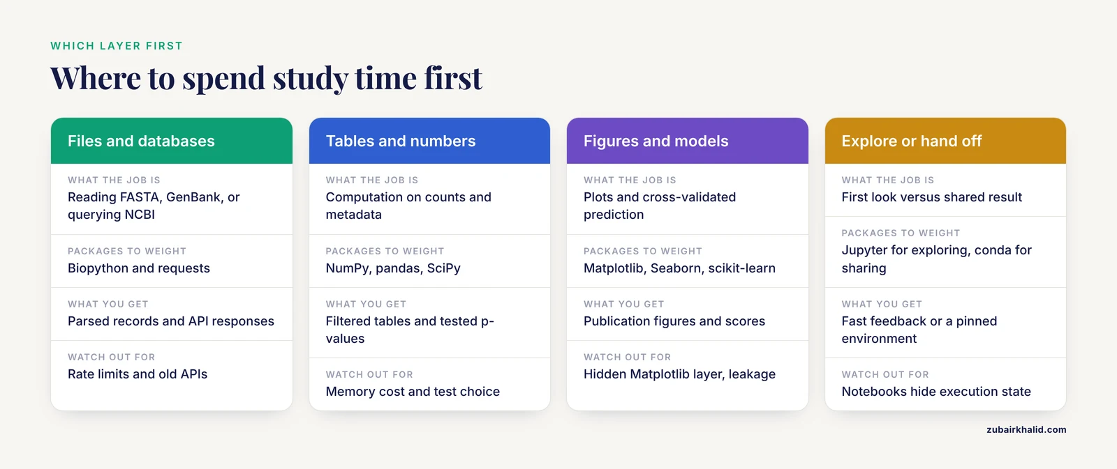
The ten packages above are not competitors, they are layers. The comparison that matters for a beginner is which layer to invest study time in first, and that comes down to four criteria.
Data format versus data analysis. Biopython and requests handle the edges of your project, where files and databases are read. NumPy, pandas, and SciPy handle the middle, where computation happens. If your first project is mostly file conversion and sequence handling, weight your study time toward Biopython. If your data already arrives as tidy CSV tables, weight it toward pandas.
Statistics versus machine learning. SciPy answers "is this difference real" with a specific hypothesis test you chose. scikit-learn answers "can a model predict this" with cross-validated performance. Recent benchmarking work underlines why the distinction matters. Neuroptimus, a platform for neuronal parameter optimization, used a common interface to compare more than twenty optimization algorithms drawn from five different Python packages across six benchmark tasks, and found that the best choice of method depended on the task [3]. The same lesson applies everywhere in Python for bioinformatics: overlapping libraries exist because methods differ, so benchmark on your own data rather than assuming one tool is universally best.
Exploration versus production. Jupyter wins for the first look, Matplotlib and Seaborn win for the figure you show, and conda wins for the environment you hand to someone else. A beginner mistake is trying to make one tool do all three jobs.
Speed versus convenience. Biopython and pandas are convenient and sometimes slow. NumPy and command-line tools are fast and less forgiving. Start convenient, profile, and optimize only the part that is actually slow.
Worked Scenarios
Scenario one: you have 200 FASTA files of 16S ribosomal RNA sequences and need length filtering and GC content per file. Biopython's SeqIO parses each file in a few lines, NumPy computes the composition, and pandas collects the per-file results into one summary table. No other packages are needed.
Scenario two: you receive a differential expression results table and want to know whether the significant genes cluster by pathway. pandas loads and filters the table, Seaborn draws a clustered heatmap of the top genes, and if you go further, a pathway-level framework applies. Method choice again matters: a benchmark of single-sample pathway analysis methods in metabolomics found that GSEA-based and z-score approaches performed better on recall while clustering and dimensionality-reduction approaches gave higher precision at moderate-to-high effect sizes [4], so read the method comparisons in any package you adopt.
Scenario three: you need to compare the outputs of two published analysis tools before trusting either. This is a real and growing pattern. MetaMutationalSigs was built for exactly this in the mutational signature field, aggregating and visually comparing refitting results from different packages because the tools produce significantly different answers [5]. The transferable lesson is to never adopt a single tool's output uncritically when multiple implementations exist.
A Five-Minute Biopython Tutorial
Here is a complete, minimal biopython tutorial exercise that combines four of the ten packages and produces a real result: fetch a RefSeq mRNA record from NCBI, compute its GC content, and plot codon usage.
from Bio import Entrez, SeqIO
import numpy as np
import pandas as pd
import matplotlib.pyplot as plt

Entrez.email = "[email protected]"   # NCBI asks you to identify yourself

handle = Entrez.efetch(db="nucleotide", id="NM_000546",
                       rettype="fasta", retmode="text")
record = SeqIO.read(handle, "fasta")
print(record.id, len(record.seq))

from Bio.SeqUtils import gc_fraction
print(round(gc_fraction(record.seq) * 100, 1))   # GC content in percent

# Codon counts across the coding sequence
seq = record.seq
codons = [str(seq[i:i+3]) for i in range(0, len(seq) - 2, 3)]
counts = pd.Series(codons).value_counts().head(10)

counts.plot(kind="bar", color="steelblue")
plt.ylabel("Count")
plt.title("Ten most frequent codons")
plt.tight_layout()
plt.savefig("codons.pdf")
Walking through it: Entrez.efetch retrieves the record, SeqIO.read parses it into a SeqRecord with an identifier and a sequence, gc_fraction returns composition as a fraction which you multiply by 100 for percent, plain slicing extracts codons, and pandas plus Matplotlib produce the figure. Every step generalizes. Replace the accession, loop over a list of identifiers, and you have a small pipeline.
Two cautions apply. Set Entrez.email before any request, both because NCBI requests it and because scripts without it are likelier to be throttled. And when you later need rigorous alignments, use Biopython's PairwiseAligner, the current alignment interface, rather than code copied from tutorials more than a few years old.
Beyond the Core Ten: Specialist Packages Worth Knowing
Once the core stack is installed, the specialist ecosystem is where bioinformatics gets interesting. None of these belongs in a beginner's first week, but knowing they exist shapes what you attempt.
Phylogenetics and comparative genomics. Profylo is an open-source Python 3 package for phylogenetic profiling, the analysis of presence-absence patterns of orthologs across species to infer functional associations between genes. It implements seven profile-comparison methods, four algorithms for identifying co-evolving gene clusters, and visualization tools, and it ships with benchmarks on human gene datasets [6]. If your interest is gene function prediction from comparative data, this is a model of what a focused specialist package looks like.
Text mining and ontologies. pyMeSHSim handles biomedical named entity recognition and semantic similarity between MeSH terms, using MetaMap to map free text to Unified Medical Language System concepts and then comparing those concepts with information-content and graph-based algorithms. In a curation of 461 GWAS phenotypes it reached recall above 0.94, precision above 0.56, and F1 above 0.70, outperforming the comparison tools DNorm and TaggerOne on MeSH recognition [7]. Note its practical dependency: it requires the external MetaMap tool, which is a realistic preview of how bioinformatics packages often wrap non-Python components.
Variant effect and high-throughput assays. sortscore scores Sort-seq experiments, a form of multiplexed assay of variant effect (MAVE) where fluorescence-activated cell sorting combined with sequencing links variants to measured phenotypes. It computes variant activity scores directly from binned counts without fitting a landscape model, handles normalization across samples, replicates, and tiled oligos, and includes heatmap visualization. The authors designed it explicitly to lower the barrier to entry, and it was used to analyze deep mutational scanning experiments for the transcription factor GLI2 [8]. It is a good example of a package that takes a beginner-friendly position on a methods debate rather than adding another model.
Pharmacokinetics and modeling. PKPy automates population pharmacokinetic analysis with minimal manual parameter initialization. In simulation studies it achieved parameter bias below 3 percent for clearance and volume of distribution in one-compartment models, identified true covariate relationships with 100 percent accuracy across tested scenarios, and maintained R squared of 0.97 or higher for model fit [9]. For anyone entering quantitative pharmacology from a Python starting point, it shows how a framework can encode rigorous defaults so beginners avoid the classic error of hand-tuning starting parameters badly.
Systems biology and metabolic models. Two packages illustrate this domain. Antimony provides a human-readable language for defining biochemical network models that converts to and from SBML, the community-standard Systems Biology Markup Language, with official bindings for Python among other languages, and its version 3 release extends support to SBML Level 3 features including flux balance constraints and probability distributions [10]. GEMsembler tackles genome-scale metabolic models (GEMs), the large reconstructions of an organism's entire metabolism: because automatic reconstruction tools produce models with different strengths, GEMsembler compares cross-tool models, tracks the origin of every feature, and builds consensus models, and its curated consensus models built from automatically reconstructed inputs outperformed gold-standard models on auxotrophy and gene essentiality predictions [11].
Transcriptomics and perturbation data. The TransPro framework pairs a Python package for interaction-aware gene selection with an R package for standardized enrichment and visualization workflows [2]. At the emerging frontier, PxFquery applies large language model assistance to functional analysis, converting over 500,000 Connectivity Map perturbation signatures into a compact functional response space so that natural-language questions can retrieve experimental perturbation evidence, with outputs that agreed more closely with experimental reference rankings than direct or PubMed-augmented LLM approaches [12]. Treat LLM-mediated tools as an area to watch rather than a beginner dependency, since the methods are young.
Optimization and method benchmarking. Finally, the Neuroptimus platform demonstrates a pattern you will encounter repeatedly: many domains now have several competing Python implementations of the same method class, and rigorous comparison requires a common interface. Neuroptimus compared more than twenty algorithms from five Python packages across six neuronal parameter search benchmarks, measuring both solution quality and convergence speed [3]. When you face several packages claiming to solve your problem, that benchmark-first mindset is the correct response, and it is a skill worth building early.
Reproducibility: Keep Your Workflows Honest
Reproducibility deserves its own section because it is the habit that separates a throwaway script from a scientific result. The core practice for a beginner is the pinned environment file described earlier. The next level is containerization, packaging software with all its dependencies so results do not depend on which versions happen to be installed. This matters because tools are updated to fix bugs and add features, and identical code can therefore produce different results on different machines or months apart [1].
You do not need to become a DevOps engineer on day one. What you need now is the discipline that makes later containerization trivial: one environment per project, versions recorded, and every download or database query written as code rather than performed by hand in a browser. The comparison tools literature points the same direction. MetaMutationalSigs, built to aggregate results across mutational signature refitting packages, is distributed as a Docker image precisely so that users get one consistent software environment rather than a fragile collection of per-tool installations [5]. Whenever you adopt a specialist package, check whether the authors provide a container or a locked environment file, and prefer those routes.
Common Mistakes and Limitations
These are the errors that cost beginners the most time, listed so you can skip them.
- Installing into the system Python. Every package on this list should live inside a conda environment. A single global environment that mixes projects guarantees a dependency conflict eventually.
- Mixing pip and conda carelessly. When both offer a package, prefer conda-forge. Reserve pip for packages conda does not carry, and install them first in a fresh environment.
- Running tutorial code from the Python 2 era or against old library APIs. Biopython in particular has renamed and deprecated functions. Check the version you installed against the documentation version you are reading.
- Forgetting
Entrez.emailbefore NCBI queries, which risks throttling and is simply against the service's stated expectations. - Trusting a single tool's output. Specialist packages disagree with each other in real, documented ways, as comparisons of mutational signature refitting tools have shown [5]. Where multiple implementations exist, benchmark on your own data, as the optimization literature demonstrates [3].
- Skipping cross-validation with scikit-learn. An accuracy score computed on the training data is not a result. Split or cross-validate, and keep preprocessing inside the validation loop.
- Confusing exploration with production. Notebooks are for thinking, scripts and pinned environments are for the record. Refactor before you share.
- Ignoring the memory cost of pandas on large tables. Reading a multi-gigabyte matrix wholesale will exhaust a laptop's memory. Learn chunked reading or convert to more compact formats before you hit the wall.
- Collecting packages instead of finishing analyses. Ten well-understood packages carry a beginner further than forty half-learned ones. The best Python packages for bioinformatics are the ones you can use without re-reading the documentation.
One honest limitation of the toolkit itself: Python packages execute your instructions, they do not design your analysis. Choices of statistical test, normalization method, and comparison tool still require domain judgment, and a poorly chosen method will produce a confident-looking wrong answer from any package on this list.
Frequently Asked Questions
What are the best Python packages for bioinformatics?
Install Biopython, NumPy, pandas, SciPy, Matplotlib, Seaborn, scikit-learn, Jupyter, conda with Bioconda, and requests first. That core covers sequence parsing, table analysis, statistics, plotting, machine learning, environment management, and database access, and specialist packages build on it later.
Should I learn Python basics before starting bioinformatics?
Yes, a week or two of general Python (variables, loops, functions, file handling) pays for itself immediately. Bioinformatics packages assume those fundamentals, and skipping them turns every error message into a mystery.
Should I use pip or conda to install packages?
Use conda as your primary installer and pip only for packages conda does not offer. Create one environment per project, prefer conda-forge when both installers carry a package, and export an environment file so your setup is reproducible.
Is Biopython alone enough for bioinformatics work?
No. Biopython handles sequences, file formats, and database access, but tables, statistics, and plots need pandas, SciPy, and Matplotlib or Seaborn. The realistic minimum working set is Biopython plus pandas plus a plotting package inside a Jupyter notebook.
Where can I find a good Biopython tutorial?
Start with the official Biopython documentation, which includes a tutorial and cookbook covering Seq objects, SeqIO parsing, and Entrez queries. The short worked example in this article, fetching a record, computing GC content, and counting codons, is a realistic first exercise to extend.
Which packages should I add after the core ten?
Add packages only when a project demands them. Phylogenetic profiling (Profylo), variant effect scoring (sortscore), metabolic modeling (Antimony, GEMsembler), and pathway analysis frameworks are the common next steps, and each is worth reading the methods behind before installing.
Sources
- FairFlow: A transparency-first framework for verifiable and reproducible bioinformatics.
- Comparative evaluation of gene selection approaches in transcriptomics: bias correction and visualization with TransPro.
- Evaluation and comparison of methods for neuronal parameter optimization using the Neuroptimus software framework.
- Single sample pathway analysis in metabolomics: performance evaluation and application.
- MetaMutationalSigs: comparison of mutational signature refitting results made easy.
- Profylo: A Python Package for Phylogenetic Profile Comparison and Analysis.
- pyMeSHSim: an integrative python package for biomedical named entity recognition, normalization, and comparison of MeSH terms.
- sortscore: Sort-seq MAVE scoring and visualization using Python.
- PKPy: a Python-based framework for automated population pharmacokinetic analysis.
- Antimony 3: Extending human-readable model definitions for SBML Level 3 Core and Packages.
- GEMsembler: consensus model assembly and structural comparison of genome-scale metabolic models across tools improve functional performance.
- PxFquery: A Bioinformatics Tool for Large Language Model-Assisted Functional Analysis of Large-Scale Perturbation Signatures.