What Is Y-Hat? Predicted Values in Regression Explained

By Dr. Zubair Khalid, DVM, MS, PhD · 2026-10-03

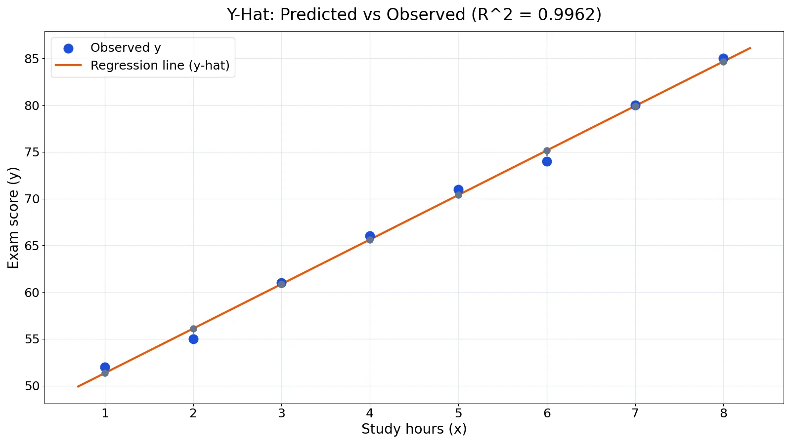
Y-hat is the value a regression equation predicts for a given input. If you fit a line to data, the equation produces one y-hat for every x you feed it. The observed y is what actually happened, and the gap between the two is the residual.

Quick Answer

Y-hat ($\hat{y}$) is the predicted or fitted value of the outcome variable from a regression model [1].
It comes from plugging an x value into the fitted equation, such as $\hat{y} = 46.5714 + 4.7619x$ in the example below.
Observed y is the real data point. Y-hat is the model's best guess at that point.
The difference $y - \hat{y}$ is the residual, which measures how far the model missed [2].
Y-hat exists for any x you choose, including values never observed in your data.

What Y-Hat Means

In plain terms, y-hat is the number your model predicts. You give it an input, it returns an output. The hat symbol is standard statistical notation for "estimated" or "predicted," so $\hat{y}$ is read as "y-hat."

The precise definition: for a set of observations $(x_i, y_i)$, a fitted regression model defines a prediction function $f$. The predicted value for observation $i$ is $\hat{y}_i = f(x_i)$, and the residual is $e_i = y_i - \hat{y}_i$ [2]. In least squares regression, the coefficients are chosen so the sum of squared residuals is as small as possible. That is the whole idea behind OLS regression.

One distinction matters early. A model can predict the mean of the response, the median, or a quantile, depending on what you are estimating [3]. Ordinary least squares targets the conditional mean, so y-hat is an estimate of the average y at that x, not a guarantee about any single case.

How It Works

For simple linear regression, the prediction equation is:

$$\hat{y} = b_0 + b_1 x$$

Each symbol means something specific:

$\hat{y}$ is the predicted value of the outcome for a given x.
$b_0$ is the intercept, the predicted y when x equals zero.
$b_1$ is the slope, the predicted change in y for a one-unit increase in x [1].
$x$ is the value of the predictor you are plugging in.

The coefficients come from the data. The slope is $b_1 = S_{xy} / S_{xx}$, where $S_{xy}$ is the sum of products of deviations and $S_{xx}$ is the sum of squared deviations of x. The intercept is $b_0 = \bar{y} - b_1\bar{x}$. Once you have both, prediction is just arithmetic.

The same logic extends to multiple predictors. With two inputs the equation becomes $\hat{y} = b_0 + b_1x_1 + b_2x_2$, and each coefficient still reflects the change in the response for a one-unit change in that factor, holding the others fixed [1]. The mechanics of computing predicted values do not change when you add terms [4].

Worked Example

The dataset is 8 students, with hours studied and exam score.

Hours (x)	Score (y)
1	52
2	55
3	61
4	66
5	71
6	74
7	80
8	85

The intermediate quantities:

n = 8
Mean of x = 4.5000
Mean of y = 68.0000
$S_{xx}$ = 42.0000
$S_{xy}$ = 200.0000
Slope $b_1 = 200.0000 / 42.0000 = 4.7619$
Intercept $b_0 = 68.0000 - 4.7619 \times 4.5000 = 46.5714$

So the fitted line is:

$$\hat{y} = 46.5714 + 4.7619x$$

Now compute y-hat and the residual for each observation.

x	Observed y	Y-hat	Residual ($y - \hat{y}$)
1	52	51.3333	0.6667
2	55	56.0952	-1.0952
3	61	60.8571	0.1429
4	66	65.6190	0.3810
5	71	70.3810	0.6190
6	74	75.1429	-1.1429
7	80	79.9048	0.0952
8	85	84.6667	0.3333

The fit is tight. $SSE = 3.6190$ and $SST = 956.0000$, so $R^2 = 1 - 3.6190/956.0000 = 0.9962$. About 99.6% of the variation in scores is explained by hours studied.

Here is the same computation in Python:

import numpy as np
x = np.array([1,2,3,4,5,6,7,8])
y = np.array([52,55,61,66,71,74,80,85])
b1, b0 = np.polyfit(x, y, 1)
yhat = b0 + b1 * x
print(b1, b0)  # 4.7619 46.5714
print(yhat)  # [51.3333 56.0952 60.8571 65.619 70.381 75.1429 79.9048 84.6667]

Output:

slope b1 = 4.7619
intercept b0 = 46.5714
R^2 = 0.9962
y-hat = [51.3333, 56.0952, 60.8571, 65.619, 70.381, 75.1429, 79.9048, 84.6667]
residuals = [0.6667, -1.0952, 0.1429, 0.381, 0.619, -1.1429, 0.0952, 0.3333]

How to Interpret It

Read y-hat as the model's expected value at that x. For a student who studied 5 hours, the model predicts a score of 70.3810. That is the center of the model's belief, not a promise. The actual student scored 71, so the residual is 0.6190.

Residuals carry the diagnostic weight. A positive residual means the observed value is above the prediction. A negative residual means it is below. In this dataset the residuals are small and show no clear pattern, which suggests the straight line is a reasonable fit. If residuals showed a curve, a straight line would be the wrong shape, and something like quadratic regression might fit better.

Two cautions apply to interpretation. First, y-hat estimates the conditional mean, so individual observations scatter around it. Second, the coefficients describe association in the observed data. They do not establish that x causes y. For that distinction, see correlation vs covariance.

When to Use It (and when not to)

Use y-hat whenever you want a point prediction from a fitted model. Common cases include forecasting a numeric outcome, filling in a missing value from related variables, and comparing predicted against observed values to check fit.

Do not use y-hat outside the range of your data without care. A line fitted on 1 to 8 hours of study will happily return a prediction for 40 hours, but that number is an extrapolation with no support in the data. Do not use a linear model's y-hat when the outcome is binary. A binary outcome calls for logistic regression, where predictions are probabilities.

Also check the model's assumptions before trusting predictions. Linearity, independence, and constant variance all affect whether y-hat is meaningful, and these are covered in assumptions of linear regression.

Y-Hat vs Observed Y

The comparison is simple. Observed y is a fact. Y-hat is a model output.

Feature	Observed y	Y-hat
What it is	The actual measured value	The model's predicted value
Source	Data collection	Fitted regression equation
Symbol	$y$	$\hat{y}$
Available for new x?	No	Yes
Contains error?	Yes, random error around the true mean	Yes, estimation error in the coefficients
Used in	Fitting the model	Prediction and diagnostics

The residual $y - \hat{y}$ is the bridge between them. It is the only place where both appear together, and it is what least squares minimizes in squared form [2].

Common Mistakes

Confusing y-hat with observed y. The fix is to check the hat. If there is no hat, it is a data value, not a prediction.
Reporting y-hat as a certainty. The fix is to report a prediction interval alongside the point estimate, since y-hat is a mean estimate and individual values vary around it.
Extrapolating far beyond the observed x range. The fix is to state the range of x used to fit the model and stay inside it.
Ignoring residual patterns. The fix is to plot residuals against fitted values. Structure in that plot means the model form is wrong.
Assuming a high $R^2$ means the predictions are accurate for new data. The fix is to check performance on held-out data, since a model can fit the training set well and still generalize poorly.
Forgetting that y-hat depends on the model. The fix is to name the model when you report a predicted value, because a different specification gives a different y-hat.

Limitations

Y-hat is only as good as the model behind it. A misspecified model produces predictions that look precise but are systematically wrong. Adding more terms always reduces residuals on the fitting data, which can create the illusion of a better model while actually increasing variance and reducing parsimony [4].

Y-hat also says nothing about uncertainty by itself. A single predicted number hides the fact that predictions have a distribution. For any real decision, pair the point prediction with an interval. And remember that a model fitted on one population may not transfer to another, so predictions outside the original context deserve skepticism.

Frequently Asked Questions

What does y-hat mean in statistics?

Y-hat is the predicted value of the dependent variable from a fitted model. The hat symbol marks it as an estimate rather than an observed data point. You get it by plugging an x value into the regression equation [1].

How do you calculate y-hat?

Multiply the slope by x, then add the intercept. In the example here, $\hat{y} = 46.5714 + 4.7619x$, so at x = 5 the prediction is 70.3810. Software like Python's numpy.polyfit returns the same coefficients.

What is the difference between y-hat and y?

Observed y is the value you measured. Y-hat is the value the model predicts for the same case. Their difference is the residual, and least squares regression chooses coefficients that minimize the sum of squared residuals [2].

Can y-hat be negative?

Yes, if the model allows it. A linear equation can return negative predictions even when the outcome cannot be negative in reality, such as a count or a price. That is a sign the model form may be wrong for the data.

Is y-hat the same as a fitted value?

Yes. Predicted value and fitted value are two names for the same quantity. Some software calls it y_pred, others call it fitted.values, but both refer to $\hat{y}$ [3].