Texas Sharpshooter Fallacy: Definition and Examples
By Dr. Zubair Khalid, DVM, MS, PhD ·
The Texas sharpshooter fallacy is naming a pattern after you have already seen the data, then treating that pattern as if you predicted it. You find a cluster, a subgroup, or a surprising result, and you build your explanation around it. The problem is that the explanation was chosen to fit the result, so the result no longer counts as evidence for it.
Quick Answer
- The fallacy takes its name from a story about a shooter who fires at a barn wall, then paints a target around the tightest cluster of holes and claims to be a marksman.
- Statistically, it means testing a hypothesis suggested by the same data you use to test it.
- Clusters appear in random data all the time, especially when you look at many groups or many outcomes.
- The fix is to state the hypothesis before you look, or to correct for the number of comparisons you made.
- It is closely related to p-hacking, multiple comparisons, and post hoc subgroup analysis.
What Texas Sharpshooter Means
In plain terms, the Texas sharpshooter fallacy is the mistake of drawing the target after the shots are fired. You look at a set of results, notice that some of them bunch together, and then declare that the bunching was the point all along. The cluster looks meaningful because you defined "meaningful" as "wherever the cluster happens to be."
The precise statistical definition is this. A hypothesis is generated from a dataset and then tested against that same dataset, without accounting for the search. The reported p-value describes the probability of seeing a result at least this extreme if the null hypothesis were true and the test had been specified in advance. When the test was chosen because of the data, that probability no longer applies. The nominal p-value understates the true false-positive rate.
This is why a study can report a small p-value and still be weak evidence. The number is real. The interpretation is wrong.
How It Works
The mechanism is easiest to see with the maximum of many observations. Suppose you have $n$ independent measurements drawn from a normal distribution with mean $\mu$ and standard deviation $\sigma$. You pick the largest one and test whether it is unusual.
The z-score of the maximum is
$$z_{\max} = \frac{x_{\max} - \bar{x}}{s}$$
where $x_{\max}$ is the largest observed value, $\bar{x}$ is the sample mean, and $s$ is the sample standard deviation. Under the null hypothesis that all values come from the same distribution, the expected value of the largest z-score is not zero. It grows with the number of observations:
$$E[z_{\max}] \approx \sqrt{2 \ln n}$$
For $n = 20$, that is $\sqrt{2 \ln 20} = 2.4477$. This formula is an asymptotic approximation that overstates the maximum for small samples. For $n = 20$ the exact expected maximum of standard normal values is about 1.87, so even when nothing is going on, the biggest of 20 values typically sits close to 2 standard deviations above the mean. If you test only that value against a threshold of 1.96, you will call it significant roughly 40% of the time by chance alone.
The Bonferroni correction is one simple guard. You divide your significance level by the number of tests:
$$\alpha_{\text{Bonferroni}} = \frac{\alpha}{n}$$
With $\alpha = 0.05$ and $n = 20$, the corrected threshold is $0.0025$. A result has to clear that bar to count as surprising once you admit you looked at 20 things.
Worked Example
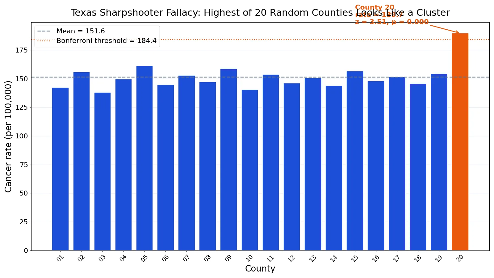
The dataset below holds simulated cancer rates per 100,000 people for 20 counties. The values were generated to show how a single high county can look alarming when it is really the maximum of a modest sample.
| County | Rate per 100k |
|---|---|
| County 01 | 142.3 |
| County 02 | 155.8 |
| County 03 | 138.1 |
| County 04 | 149.6 |
| County 05 | 161.2 |
| County 06 | 144.7 |
| County 07 | 152.9 |
| County 08 | 147.3 |
| County 09 | 158.4 |
| County 10 | 140.5 |
| County 11 | 153.6 |
| County 12 | 146.2 |
| County 13 | 150.8 |
| County 14 | 143.9 |
| County 15 | 156.7 |
| County 16 | 148.1 |
| County 17 | 151.4 |
| County 18 | 145.6 |
| County 19 | 154.3 |
| County 20 | 189.7 |
Here are the steps, using the computed values.
- Sample size: $n = 20$.
- Mean rate: $3031.1 / 20 = 151.5550$.
- Sample standard deviation: $s = 10.8725$.
- Highest county: County 20 with a rate of 189.7.
- Z-score of the maximum: $(189.7 - 151.5550) / 10.8725 = 3.5084$.
- Two-sided p-value: $2 \times (1 - \Phi(3.5084)) = 0.0005$.
- Bonferroni alpha: $0.05 / 20 = 0.0025$.
- Bonferroni critical z: $z_{\text{crit}} = 3.0233$.
- Bonferroni threshold rate: $151.5550 + 3.0233 \times 10.8725 = 184.4264$.
- Approximate expected maximum z under the null (asymptotic formula): $\sqrt{2 \ln 20} = 2.4477$. The exact value for 20 normal draws is about 1.87.
The uncorrected test flags County 20 as significant, and it also clears the Bonferroni threshold of 184.4264. That is a useful contrast with the usual Texas sharpshooter story. Correction does not automatically erase every finding. It raises the bar, and here the maximum still clears it. What changes is the claim you are allowed to make. You can say County 20 is high relative to the others after accounting for the search. You cannot say you knew County 20 would be high before you looked.
The same logic runs in Python:
import numpy as np
from scipy import stats
rates = [142.3, 155.8, 138.1, 149.6, 161.2, 144.7, 152.9, 147.3, 158.4, 140.5, 153.6, 146.2, 150.8, 143.9, 156.7, 148.1, 151.4, 145.6, 154.3, 189.7]
n = len(rates)
z = (max(rates) - np.mean(rates)) / np.std(rates, ddof=1)
p = 2 * (1 - stats.norm.cdf(abs(z)))
alpha_bonf = 0.05 / n
print(f"z = {z:.4f}, p = {p:.4f}, Bonferroni alpha = {alpha_bonf:.4f}")
Output:
z = 3.5084, p = 0.0005, Bonferroni alpha = 0.0025In a spreadsheet, the mean is =AVERAGE(B2:B21), the standard deviation is =STDEV.S(B2:B21), the z-score is =(B21-AVERAGE(B2:B21))/STDEV.S(B2:B21), the p-value is =2*(1-NORM.S.DIST(ABS((B21-AVERAGE(B2:B21))/STDEV.S(B2:B21)),TRUE)), and the Bonferroni alpha is =0.05/20.
How to Interpret It
When you see a striking cluster, ask three questions. First, how many groups or outcomes were examined before this one was chosen? Second, was the hypothesis written down before the data arrived? Third, does the reported uncertainty account for the search?
If the answer to the first question is "many" and the second is "no," treat the finding as a lead, not a conclusion. A cluster is a reason to run a fresh study, not a reason to announce an effect.
The expected maximum formula gives you a quick sanity check. If your "surprising" result is close to $\sqrt{2 \ln n}$ standard deviations from the mean, it is about what random noise would produce. That does not prove the result is spurious. It tells you the result is not surprising on its own.
When to Use It (and when not to)
Use the Texas sharpshooter lens whenever a claim rests on a pattern discovered in the data. This covers post hoc subgroup analysis in clinical trials, hotspot mapping in epidemiology, gene association scans, and any dashboard where someone circles the one metric that moved.
Do not use it to dismiss every unexpected finding. Exploratory analysis is legitimate and valuable. The error is not in noticing the pattern. The error is in reporting the p-value as if the pattern had been predicted. If you label the work as exploratory and follow up with a confirmatory test on new data, you have avoided the fallacy.
One source notes that an observational study design can sidestep some of this concern, since the researchers are not assigning treatments and the analysis is descriptive [1]. Another discusses a study where no explicit hypothesis was stated, and argues the results should be taken with a grain of salt for that reason [2]. Both point at the same issue. The credibility of a finding depends on whether the question came before the answer.
Texas Sharpshooter vs P-Hacking
The two overlap heavily, but they are not identical. P-hacking is the behavior. The Texas sharpshooter fallacy is the reasoning error that makes the behavior look acceptable.
| Feature | Texas Sharpshooter Fallacy | P-Hacking |
|---|---|---|
| Core idea | Target drawn after the shots | Tests run until one is significant |
| Main problem | Hypothesis chosen from the data | Selective reporting of results |
| Typical setting | Clusters, hotspots, subgroups | Many outcomes or stopping rules |
| Fix | Pre-register the hypothesis | Report all tests, correct for multiplicity |
| Relationship | The fallacy is the justification | P-hacking is the practice |
You can commit the Texas sharpshooter fallacy without p-hacking if you simply eyeball a map and invent a story. You can p-hack without framing it as a prediction. In practice they usually travel together.
Common Mistakes
- Testing the maximum and reporting it as a planned test. Fix: state how many groups you compared and apply a multiplicity correction such as Bonferroni.
- Treating a subgroup result as if it were the primary outcome. Fix: label subgroup analyses as exploratory and confirm them in a separate sample.
- Ignoring the base rate of clusters. Fix: compare your cluster's z-score to the expected maximum, $\sqrt{2 \ln n}$, before calling it unusual.
- Confusing statistical significance with a pre-specified hypothesis. Fix: check whether the hypothesis existed before the data was collected.
- Correcting for multiplicity only when it suits the story. Fix: decide the correction method before analysis and apply it consistently.
- Assuming correction always kills the finding. Fix: run the corrected test. In the worked example, the maximum still cleared the Bonferroni threshold.
Limitations
The Texas sharpshooter framing tells you when a p-value is untrustworthy. It does not tell you whether the underlying effect is real. A cluster can survive correction and still be caused by confounding, measurement error, or a genuine local factor. Correction addresses the search, not the study design.
The methods used to guard against it have their own costs. Bonferroni is conservative when tests are correlated, which is common in spatial and genomic data. It can hide real effects. Other approaches, such as permutation tests or hierarchical models, handle dependence better but require more assumptions and more data. No correction can rescue a study where the hypothesis was invented after seeing the results and never tested again.
Frequently Asked Questions
What is the Texas sharpshooter fallacy in simple terms?
It is drawing the target around the bullet holes after you shoot. You find a pattern in data, then act as if you predicted that pattern. The name comes from a story about a shooter who fires at a barn and then paints a bullseye around the tightest cluster.
Why is it called the Texas sharpshooter fallacy?
The name comes from a folk story about a Texan who fires randomly at a barn wall, then paints a target around the densest cluster of holes and claims to be a great shot. The story is a parable, not a documented event. It captures the idea of defining success after seeing the outcome.
How is it related to p-hacking?
P-hacking is running many tests or trying many analyses until one produces a small p-value. The Texas sharpshooter fallacy is the reasoning that makes the resulting p-value look meaningful. Both ignore the fact that the hypothesis was chosen because of the data.
How do I avoid the Texas sharpshooter fallacy?
Write your hypothesis before you look at the data. If you must explore, say so and treat the results as leads. When you compare many groups, correct for the number of comparisons. Then confirm the finding on a fresh dataset.
Does a Bonferroni correction always remove the effect?
No. It raises the threshold for significance. In the worked example, the highest county had a z-score of 3.5084, which still exceeded the Bonferroni critical value of 3.0233. Correction changes what you can claim, not necessarily whether the result stands.
References
- Are Certain People More Prone to Addiction? | SiOWfa16: Science in Our World: Certainty and Controversy
- experiment | SiOWfa13: Science in Our World
Further Reading
- Wilson G, Bryan J, Cranston K et al. (2017). Good enough practices in scientific computing. PLOS Computational Biology
- Wilkinson MD, Dumontier M, Aalbersberg IJ et al. (2016). The FAIR Guiding Principles for scientific data management and stewardship. Scientific Data
- NIST/SEMATECH e-Handbook of Statistical Methods
- Broman KW, Woo KH (2018). Data Organization in Spreadsheets. The American Statistician