Normal CDF: Definition, Formula and Calculator Examples
By Dr. Zubair Khalid, DVM, MS, PhD ·
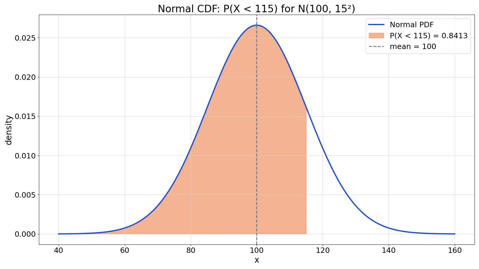
The normal CDF (cumulative distribution function) gives the probability that a normally distributed variable takes a value less than or equal to some number $x$. It equals the area under the normal curve to the left of $x$, and it is the tool you use for questions like "what fraction of students scored below 115?" You can compute it with a table, a calculator, Excel, or Python.
Quick Answer
- The normal CDF is $F(x) = P(X \le x)$, the left-tail area under a normal curve.
- For a general normal distribution, standardize first: $z = (x - \mu)/\sigma$, then use the standard normal CDF $\Phi(z)$.
- The standard normal CDF has no simple closed form, so it is computed numerically [1].
- On a TI-84, press [2nd] [DISTR], choose 2:normalcdf, and enter lower, upper, mean, and standard deviation [2].
- In Excel,
=NORM.DIST(x, mean, sd, TRUE)returns the same value.
What the Normal CDF Means
The cumulative distribution function of a random variable $X$ at a point $x$ is the probability that $X$ takes on a value less than or equal to $x$ [3]. In symbols, $F(x) = P(X \le x)$.
For a normal distribution, that probability is the area under the bell curve to the left of $x$. The total area under the curve is 1, so the CDF runs from 0 on the far left to 1 on the far right. At the mean, the CDF equals 0.5, because half the area sits on each side.
The standard normal distribution is the special case with mean $\mu = 0$ and standard deviation $\sigma = 1$ [1]. Its CDF is written $\Phi(z)$ and is the version tabulated in textbooks. Any normal distribution can be converted to this one by subtracting the mean and dividing by the standard deviation, which is why one table or one calculator function covers every normal problem [4].
How It Works
The CDF of the standard normal distribution is the integral of its probability density function from negative infinity to $x$ [1]:
$$F(x) = \int_{-\infty}^{x} \frac{e^{-x^{2}/2}}{\sqrt{2\pi}} \, dx$$
That integral does not exist in a simple closed formula, so it is computed numerically [1]. For a normal distribution with mean $\mu$ and standard deviation $\sigma$, you standardize first:
$$z = \frac{x - \mu}{\sigma}, \qquad P(X \le x) = \Phi(z)$$
Each symbol means the following.
| Symbol | Meaning |
|---|---|
| $x$ | The value you are asking about |
| $\mu$ | Mean of the distribution |
| $\sigma$ | Standard deviation of the distribution |
| $z$ | Standard score, the number of standard deviations $x$ sits from the mean |
| $\Phi(z)$ | Standard normal CDF, the area left of $z$ |
| $F(x)$ | CDF of the original normal variable |
For an interval, subtract two CDF values. The probability that $X$ falls between $a$ and $b$ is $P(a < X < b) = F(b) - F(a)$ [5]. This works because the area left of $b$ contains the area left of $a$, so the difference leaves only the strip between them.
If you want the density curve itself instead of the accumulated area, see Normal PDF: Formula, Definition and Examples. The difference between the two functions is covered in CDF vs PDF: Differences and When to Use Each.
Worked Example
Suppose exam scores in a large course are normally distributed with a mean of 100 and a standard deviation of 15. You want the probability that a randomly chosen student scored below 115, and the probability of a score between 90 and 120.
The steps below use the computed values for this distribution.
| Step | Calculation | Result |
|---|---|---|
| Standardize $x = 115$ | $z = (115 - 100) / 15$ | 1.0000 |
| Left-tail probability | $\Phi(1.0000)$ | 0.8413 |
| Standardize $x = 90$ | $z = (90 - 100) / 15$ | -0.6667 |
| Standardize $x = 120$ | $z = (120 - 100) / 15$ | 1.3333 |
| Interval probability | $0.9088 - 0.2525$ | 0.6563 |
So $P(X < 115) = 0.8413$ and $P(90 < X < 120) = 0.6563$. About 84 percent of students score below 115, and about 66 percent score between 90 and 120.
The same numbers come out of Python and Excel.
from scipy import stats
mu, sigma = 100, 15
p1 = stats.norm.cdf((115 - mu) / sigma)          # 0.8413
p2 = stats.norm.cdf((120 - mu) / sigma) - stats.norm.cdf((90 - mu) / sigma)  # 0.6563
print(f"P(X < 115) = {p1:.4f}")
print(f"P(90 < X < 120) = {p2:.4f}")
Output:
P(X < 115) = 0.8413
P(90 < X < 120) = 0.6563
For a second view of the same idea, here is a small dataset of 15 exam scores.
| student_id | score |
|---|---|
| 1 | 88 |
| 2 | 92 |
| 3 | 105 |
| 4 | 97 |
| 5 | 113 |
| 6 | 101 |
| 7 | 95 |
| 8 | 108 |
| 9 | 99 |
| 10 | 110 |
| 11 | 103 |
| 12 | 91 |
| 13 | 117 |
| 14 | 96 |
| 15 | 104 |
This sample has a mean of 101.2667 and a standard deviation of 8.4046. Those are sample statistics, not the population parameters used in the probability calculation above. The distinction matters, and it is explained in Mean and Standard Deviation: Definition, Formula and Examples.
How to Interpret It
A CDF value is a probability, so it always sits between 0 and 1. Read it as the share of the distribution at or below your value. A result of 0.8413 means roughly 84 percent of the distribution lies to the left of $x$.
Because the normal curve is symmetric, a few reference points are worth memorizing. The CDF at the mean is 0.5. One standard deviation above the mean gives about 0.84, two gives about 0.98. One standard deviation below the mean gives about 0.16.
To get a right-tail probability, subtract from 1. The probability that $X$ is greater than $x$ is $1 - F(x)$. To get an interval, subtract the smaller CDF from the larger one [5].
When to Use It (and when not to)
Use the normal CDF when your variable is approximately normally distributed and you want a probability or a proportion. Typical cases include measurement error, heights, test scores, and sample means from reasonably large samples. It is also the basis for many confidence intervals and hypothesis tests, since critical values come from the normal CDF [4].
Do not use it when the data are clearly skewed, heavy-tailed, or bounded in a way the normal curve cannot represent, such as counts or waiting times. Do not use it for discrete outcomes without a continuity correction. And do not treat a sample mean and sample standard deviation as if they were the true population parameters without accounting for that uncertainty.
If you want to skip the manual work, the Normal Distribution Calculator returns left-tail, right-tail, and interval probabilities directly.
Normal CDF vs Normal PDF
The PDF and the CDF describe the same distribution in different ways. The PDF gives the height of the curve at a point. The CDF gives the accumulated area up to that point.
| Feature | Normal PDF | Normal CDF |
|---|---|---|
| Output | Density height at $x$ | Probability $P(X \le x)$ |
| Range of values | Any positive number | 0 to 1 |
| Area meaning | Not an area by itself | Area under the curve to the left |
| Typical use | Shape, likelihood, curve plotting | Probabilities, p-values, proportions |
| Interval probability | Requires integration | Subtract two CDF values |
A single point has probability zero under a continuous distribution, so the PDF value at a point is not a probability. Only areas, which the CDF provides, are probabilities.
Common Mistakes
- Forgetting to standardize. If you plug a raw value into a standard normal table, you get nonsense. Fix: compute $z = (x - \mu)/\sigma$ first, or use a function that takes the mean and standard deviation as arguments.
- Mixing up the order in an interval. Subtracting the larger CDF from the smaller gives a negative probability. Fix: always compute $F(\text{upper}) - F(\text{lower})$.
- Using the sample standard deviation as $\sigma$. The sample value estimates the population parameter but is not the same thing. Fix: be explicit about which one you are using and why.
- Confusing left-tail and right-tail output. Some calculators and functions return the area to the left, others to the right. Fix: check the documentation, then convert with $1 - F(x)$ if needed.
- Entering the variance instead of the standard deviation. Excel's
NORM.DISTexpects the standard deviation. Fix: take the square root of the variance before entering it. - Assuming normality without checking. A histogram or a normal quantile plot is a quick check [2]. Fix: plot the data before trusting a normal-based probability.
Limitations
The normal CDF only describes normal distributions. Real data are often skewed, have outliers, or are bounded, and forcing a normal model onto them produces probabilities that look precise but are wrong. The normal curve also extends infinitely in both directions, so it assigns nonzero probability to impossible values such as negative heights or negative times.
The function itself is computed numerically, not from a closed formula [1], so results depend on the precision of the table, calculator, or software you use. Tables typically round to four or five decimals, which is fine for most work but not for very small tail probabilities. For extreme tails, use software rather than a printed table.
Frequently Asked Questions
What does normal cdf mean on a calculator?
On a TI-84, normalcdf is the cumulative distribution function for a normal distribution. You give it a lower bound, an upper bound, the mean, and the standard deviation, and it returns the probability that a value falls between those bounds [2]. If you leave out the mean and standard deviation, it uses the standard normal distribution with mean 0 and standard deviation 1 [2].
How do I find the normal CDF by hand?
Standardize your value with $z = (x - \mu)/\sigma$, then look up $z$ in a standard normal table. The table gives the area from 0 to $z$, so add 0.5 for a positive $z$ to get the full left-tail probability [4]. For negative values, use $P(X \le a) = 1 - P(X \le |a|)$ [4].
What is the difference between normal cdf and normal pdf?
The PDF gives the height of the density curve at a point, and its value is not a probability. The CDF gives the probability that the variable is less than or equal to a point, which is the area under the curve to the left [3]. Use the PDF to describe shape and the CDF to compute probabilities.
How do I find the probability between two values?
Compute the CDF at the upper value and the CDF at the lower value, then subtract. For example, $P(90 < X < 120) = F(120) - F(90) = 0.9088 - 0.2525 = 0.6563$ for a normal distribution with mean 100 and standard deviation 15 [5].
Can I use the normal CDF in Excel?
Yes. =NORM.DIST(x, mean, sd, TRUE) returns the cumulative probability up to $x$. Set the last argument to TRUE for the CDF and FALSE for the PDF. For an interval, subtract two calls, as in =NORM.DIST(120,100,15,TRUE)-NORM.DIST(90,100,15,TRUE). The syntax is covered in more detail in NORM.DIST Formula in Excel: Syntax and Examples.
References
- 1.3.6.6.1. Normal Distribution
- 6.4: Normal Distribution - Statistics LibreTexts/06%3A_Continuous_Probability_Distributions/6.04%3A_Normal_Distribution)
- CS109
- 1.3.6.7.1. Cumulative Distribution Function of the Standard Normal Distribution
- normal.html