Nonlinear Relationships: Definition and Examples

By Dr. Zubair Khalid, DVM, MS, PhD · 2026-10-03

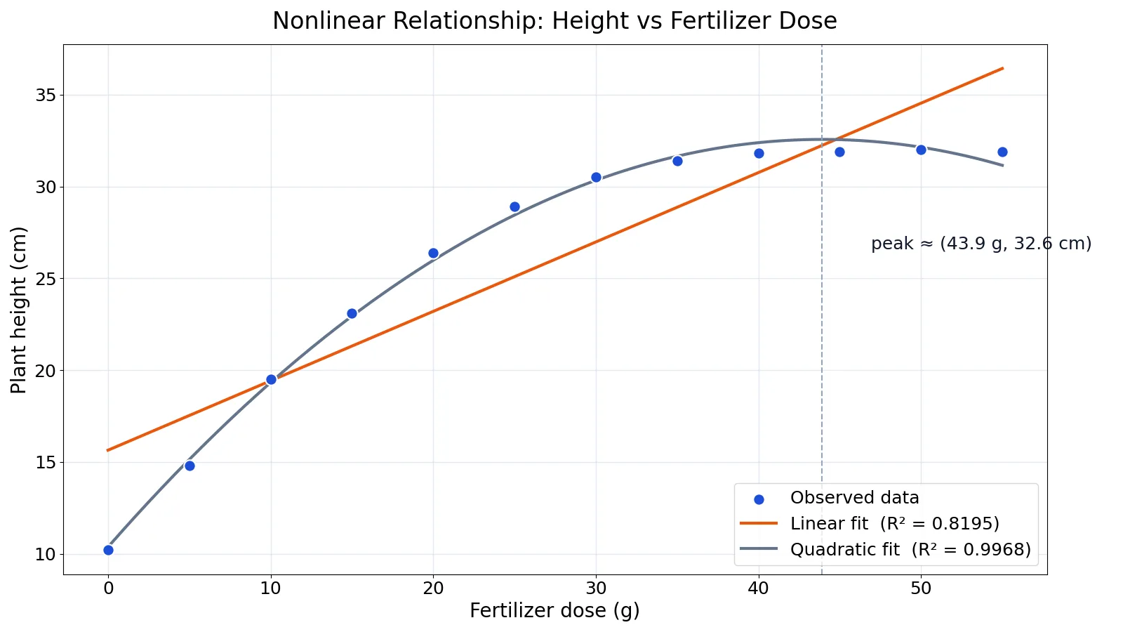
A nonlinear relationship is one where a straight line does not describe how two variables move together. The rate of change is not constant, so the graph bends, curves or flattens. You can often spot a nonlinear pattern by eye in a scatter plot, then confirm it by comparing a linear fit with a curved one.

Quick Answer

A relationship is nonlinear when a one-unit increase in the input does not always produce the same change in the output.
Nonlinear models allow parameters to enter the equation in flexible ways, so almost any function written in closed form can be used [1].
Common shapes include U-curves, inverted U-curves, exponential growth, logarithmic growth and S-curves.
A scatter plot is your first check. If the points bend away from a straight line, suspect nonlinearity.
Compare fit statistics. In the example below, a quadratic fit raises R² from 0.8195 to 0.9968.

What Nonlinear Means

In plain terms, a nonlinear relationship is any relationship that is not a straight line. If you double the input and the output does not double in a predictable, proportional way, the relationship is nonlinear.

The precise statistical definition comes from the model form. A nonlinear regression model is written as

$$ y = f(\vec{x};\vec{\beta}) + \varepsilon $$

where the function $f$ is nonlinear in the parameters $\vec{\beta}$ [1]. The key phrase is "nonlinear in the parameters." A model can have squared terms and still be linear in the parameters, which is why a quadratic fit is often called a linear model with a curved shape. True nonlinear regression covers a much larger class of functions, and unlike linear regression there are very few limits on how parameters can appear in the functional part of the model [1].

Nonlinearity also appears outside regression. In algebra, variables raised to powers or placed in denominators make an inequality nonlinear, such as $m^2 - 8m > 9$ or $\frac{x-4}{(3x-2)(x+5)} \leq 0$ [2]. In dynamical systems, a nonlinear system is often written as $\dot{\mathbf{X}}(t) = F(\mathbf{X})$ where $F$ is a nonlinear function, and such systems are difficult or impossible to solve analytically [3]. The common thread is that the output does not scale in a fixed proportion to the input.

How It Works

The mechanism is easiest to see by comparing two equations.

A linear model is

$$ y = b_0 + b_1 x $$

Here $b_0$ is the intercept, the value of $y$ when $x$ is zero. $b_1$ is the slope, the change in $y$ for each one-unit increase in $x$. That slope is the same everywhere along the line.

A quadratic model adds a squared term:

$$ y = a x^2 + b x + c $$

Here $a$, $b$ and $c$ are the coefficients. The squared term lets the curve change direction. When $a$ is negative, the curve opens downward and has a peak. When $a$ is positive, it opens upward and has a trough. The turning point, or vertex, sits at

$$ x^* = -\frac{b}{2a} $$

That single formula tells you where the relationship switches from rising to falling, or the reverse.

More general nonlinear models follow the same idea. The function $f$ can contain exponentials, logarithms, powers or ratios, and the parameters inside it are estimated by fitting the curve to the data [1]. The estimation logic is conceptually the same as linear least squares, but the curve can take far more shapes.

Worked Example

The dataset below records fertilizer dose in grams against plant height in centimeters for 12 plants. Height rises quickly at low doses, then levels off.

dose_g	height_cm
0	10.2
5	14.8
10	19.5
15	23.1
20	26.4
25	28.9
30	30.5
35	31.4
40	31.8
45	31.9
50	32.0
55	31.9

The sample size is $n = 12$ and the mean height is 26.0333 cm. The total sum of squares, which measures how much the heights vary around that mean, is $SS_{tot} = 622.9667$.

A straight line fitted to these points has slope 0.3779 and intercept 15.6410. Its residual sum of squares is $SS_{res,lin} = 112.4209$, giving

$$ R^2_{lin} = 1 - \frac{112.4209}{622.9667} = 0.8195 $$

That looks respectable. But the residuals are not random. The line overestimates height at the lowest and highest doses and underestimates it in the middle, which is the signature of a curve.

A quadratic fit returns coefficients $a = -0.0115$, $b = 1.0106$ and $c = 10.3681$. Its residual sum of squares drops to $SS_{res,quad} = 2.0161$, so

$$ R^2_{quad} = 1 - \frac{2.0161}{622.9667} = 0.9968 $$

The improvement is $0.9968 - 0.8195 = 0.1772$. The quadratic explains almost all the remaining variation.

The vertex sits at

$$ x^* = -\frac{1.0106}{2(-0.0115)} = 43.9241 \text{ g} $$

with a predicted height of 32.5641 cm. That is the dose where height peaks before flattening out.

Here is the code that produced these numbers.

import numpy as np
dose = np.array([0,5,10,15,20,25,30,35,40,45,50,55], dtype=float)
height = np.array([10.2,14.8,19.5,23.1,26.4,28.9,30.5,31.4,31.8,31.9,32.0,31.9])

lin = np.polyfit(dose, height, 1)
quad = np.polyfit(dose, height, 2)

def r2(y, yhat):
    return 1 - np.sum((y-yhat)**2)/np.sum((y-y.mean())**2)

print("R2 linear   :", round(r2(height, np.polyval(lin, dose)), 4))
print("R2 quadratic:", round(r2(height, np.polyval(quad, dose)), 4))
a, b, c = quad
x_star = -b/(2*a)
print(f"Quadratic peak at dose = {x_star:.4f} g, height = {np.polyval(quad, x_star):.4f} cm")

Output:

R2 linear   : 0.8195
R2 quadratic: 0.9968
Quadratic peak at dose = 43.9241 g, height = 32.5641 cm

How to Interpret It

Start with the shape, not the number. Plot the data. If the cloud of points bends, a straight line will leave a pattern in the residuals, and that pattern is the evidence of nonlinearity.

Then read the coefficients in context. In the example, the negative $a$ means the curve opens downward, so there is a maximum. The vertex at 43.9 g tells you the dose beyond which extra fertilizer stops adding height. That is a practical answer a linear slope of 0.3779 cm per gram cannot give you, because that slope implies height keeps rising forever.

Compare $R^2$ values with care. A jump from 0.8195 to 0.9968 is large, but adding any flexible term tends to raise $R^2$ at least a little. The size of the gain and the shape of the residuals together tell you whether the curve is real. For a deeper look at fitting curved terms, see quadratic regression analysis.

Finally, check the direction of the relationship before you describe it. A nonlinear pattern can be positive over part of its range and negative over another, which is different from a simple negative correlation.

When to Use It (and when not to)

Use a nonlinear model when theory or the scatter plot suggests a curve. Growth curves, dose-response curves, saturation effects and diminishing returns all fit this description. Nonlinear least squares can produce good estimates of unknown parameters with relatively small datasets, and it shares with linear least squares a fairly well-developed theory for computing confidence, prediction and calibration intervals [1].

Use it when the turning point itself is the answer. If you need to know the optimal dose, the peak of a curve, or the point where a trend reverses, a linear model cannot express that.

Do not reach for a nonlinear model just because it fits better. If the underlying process is genuinely linear and the bend is noise, a curve will chase that noise and predict poorly on new data. Do not use a flexible curve to paper over a small sample either. With few points, a quadratic can pass near every observation and still be wrong.

Also consider whether a transformation solves the problem more simply. A logarithmic or square-root transform can straighten some curved relationships and keep the model easy to interpret. For a broader view of how predictors and outcomes are set up, see explanatory variable and dependent variable examples.

Nonlinear vs Linear

The table below contrasts the two in the terms that matter for analysis.

Feature	Linear	Nonlinear
Shape on a scatter plot	Straight line	Curve, bend or plateau
Rate of change	Constant	Changes across the range
Model form	$y = b_0 + b_1 x$	$y = f(\vec{x};\vec{\beta})$ with $f$ nonlinear in parameters [1]
Turning points	None	Possible, found at $x^* = -b/(2a)$ for a quadratic
Example fit	R² = 0.8195	R² = 0.9968
Typical use	Steady proportional change	Growth, saturation, dose-response

The distinction is about the parameters, not the picture. A quadratic has a curved graph but is linear in its coefficients, so it is usually fitted with linear least squares. A model where a parameter sits inside an exponent is nonlinear in the stricter sense [1].

Common Mistakes

Judging by R² alone. A higher R² does not prove the curve is correct. Fix: inspect the residuals and confirm the shape matches the process.
Ignoring the scatter plot. Fitting a line to obviously curved data hides the real pattern. Fix: always plot before you model, as in this bivariate data workflow.
Extrapolating past the turning point. The quadratic peaks at 43.9 g, so predictions at 80 g are unsupported. Fix: keep predictions inside the observed dose range.
Confusing "curved graph" with "nonlinear in parameters." A quadratic bends but is linear in its coefficients. Fix: check where the parameters appear in the equation [1].
Adding terms until the fit looks good. Extra terms can fit noise. Fix: justify each term with theory or a clear pattern in the residuals.
Reading a plateau as a decline. In the example, height at 55 g is 31.9 cm, barely below the 32.0 cm at 50 g. Fix: treat small reversals as flat unless the drop is larger than the noise.

Limitations

A nonlinear fit describes the data you gave it, not the mechanism behind it. The quadratic here peaks at 43.9 g, but that number depends on the doses tested and the measurement error in each height. Change the range and the peak can move.

Interpretation of intervals is also weaker than in linear regression. In most cases the probabilistic interpretation of intervals produced by nonlinear regression is only approximately correct, though those intervals still work well in practice [1]. Nonlinear systems more generally can be difficult or impossible to solve analytically, which is why simulation and geometric analysis are often used instead [3]. Treat any single fitted curve as one plausible description among several.

Frequently Asked Questions

What is a simple definition of a nonlinear relationship?

It is a relationship where a straight line does not capture how the variables move together. The rate of change shifts as the input changes, so the graph bends, curves or flattens. If doubling the input does not produce a predictable proportional change in the output, the relationship is nonlinear.

How do I tell if my data is nonlinear?

Plot the variables against each other and look for a bend. Then fit a straight line and check the residuals. If the residuals form a pattern, such as a curve or a U-shape, the relationship is nonlinear. Comparing a linear and a curved fit, as in the fertilizer example, confirms it numerically.

Is a quadratic relationship nonlinear?

It depends on which sense you mean. The graph is curved, so it is nonlinear in shape. But a quadratic is linear in its coefficients, so it is usually estimated with linear least squares. True nonlinear regression allows parameters to appear in far more flexible ways, such as inside exponents [1].

Can a nonlinear relationship be negative?

Yes. A curve can slope downward over part or all of its range. A relationship can also be positive at low inputs and negative at high inputs, which is what happens after a peak. That is why you should describe the direction over a stated range, not for the whole curve.

Why does a nonlinear model fit better?

A flexible curve has more freedom to follow the data, so it usually fits better than a straight line. That does not automatically make it the right model. The gain matters only if the shape matches the underlying process and the residuals stop showing a pattern.

References

4.1.4.2. Nonlinear Least Squares Regression
2.2: Solving Nonlinear Inequalities - Mathematics LibreTexts/02%3A_Inequalities_and_Functions/2.02%3A_Solving_Nonlinear_Inequalities)
Nonlinear Dynamics Modeling and Control - Beyond Linear Thinking | PI: Dr. Hui Yang, Gary and Sheila Bello Chair and Professor @ Pennsylvania State Un