Multicollinearity: Definition, Detection and Examples

By Dr. Zubair Khalid, DVM, MS, PhD · 2026-10-03

Multicollinearity is a condition in regression where two or more predictor variables are highly correlated with each other. It does not stop you from fitting a model, but it makes the individual coefficient estimates unstable and hard to trust. This article explains what multicollinearity is, why it harms regression models, and how to detect it with variance inflation factors (VIF).

Quick Answer

Multicollinearity means predictor variables in a regression carry overlapping information [1].
It inflates the standard errors of coefficients, so estimates become uncertain and can even flip sign [1].
It does not bias predictions much, but it wrecks the interpretation of individual coefficients.
The standard detection tool is the variance inflation factor, computed as $VIF = 1/(1-R^2)$ [1].
A common rule of thumb is that a VIF above 5 or 10 signals a problem worth addressing.

What Multicollinearity Means

In plain terms, multicollinearity is redundancy among your predictors. If two variables move together almost perfectly, the model struggles to tell which one is doing the work. When a linear model has two or more highly correlated predictor variables, it is often said to suffer from multicollinearity [1].

The precise statistical definition is about the design matrix. In a regression with predictors $X_1, X_2, \dots, X_k$, multicollinearity exists when one predictor can be predicted well from a linear combination of the others. Perfect multicollinearity means an exact linear relationship, which makes the matrix of predictors singular and the coefficients impossible to estimate uniquely. Near-perfect multicollinearity is the practical case. The predictors are not exactly dependent, but they are close enough that the estimates become fragile.

The term "multicollinear" describes a single pair or set of variables in this state. You will see both "multicollinear" and "multicollinearity" used, and they refer to the same underlying condition.

How It Works

The core mechanism is that correlated predictors share variance, so the model cannot cleanly assign credit. The standard diagnostic is the variance inflation factor. For predictor $j$, it is:

$$VIF_j = \frac{1}{1 - R_j^2}$$

Each symbol means the following:

$VIF_j$ is the variance inflation factor for predictor $j$.
$R_j^2$ is the coefficient of determination from regressing predictor $j$ on all the other predictors.

When $R_j^2$ is 0, the predictor is unrelated to the others and $VIF_j = 1$, meaning no inflation. As $R_j^2$ approaches 1, the denominator shrinks toward 0 and the VIF grows without bound. A VIF of 5 means the variance of that coefficient is five times larger than it would be if the predictor were uncorrelated with the rest. The square root of the VIF tells you how much the standard error is inflated.

This is why multicollinearity is usually detected using variance inflation factors [1]. The same logic applies when you work with categorical predictors, where the dummy coding can itself introduce dependencies if you are careless [2].

Worked Example

The dataset is 25 house records with size (sqft), rooms, and price ($k). Size and rooms rise together, which is exactly the setup that produces multicollinearity.

size	rooms	price
1200	3	210
1350	3	235
1500	4	260
1600	4	275
1750	4	300
1800	4	310
1900	5	330
2000	5	345
2100	5	360
2200	5	375
2300	5	390
2400	6	405
2500	6	420
2600	6	435
2700	6	450
2800	6	465
2900	7	480
3000	7	495
3100	7	510
3200	7	525
3300	7	540
3400	8	555
3500	8	570
3600	8	585
3700	8	600

The steps run as follows.

Sample size $n = 25$.
Predictors $k = 2$ (size and rooms).
Correlation $r(\text{size}, \text{rooms}) = 0.9833$.
Regress size on rooms: $R^2 = 0.9669$.
$VIF(\text{size}) = 1/(1 - 0.9669) = 30.1990$.
Regress rooms on size: $R^2 = 0.9669$.
$VIF(\text{rooms}) = 1/(1 - 0.9669) = 30.1990$.
OLS $R^2$ of the full model = 0.9993.

Both predictors have a VIF of 30.1990, far above the usual threshold of 10. The full model fits the data almost perfectly, yet the individual coefficients are unreliable because size and rooms are nearly the same variable.

Here is the code that produces these numbers.

import pandas as pd, statsmodels.api as sm
from statsmodels.stats.outliers_influence import variance_inflation_factor
X = df[['size','rooms']]
Xc = sm.add_constant(X)
vif = [variance_inflation_factor(Xc.values, i) for i in range(1, Xc.shape[1])]
print(f"VIF(size)={vif[0]:.4f}, VIF(rooms)={vif[1]:.4f}")

Output:

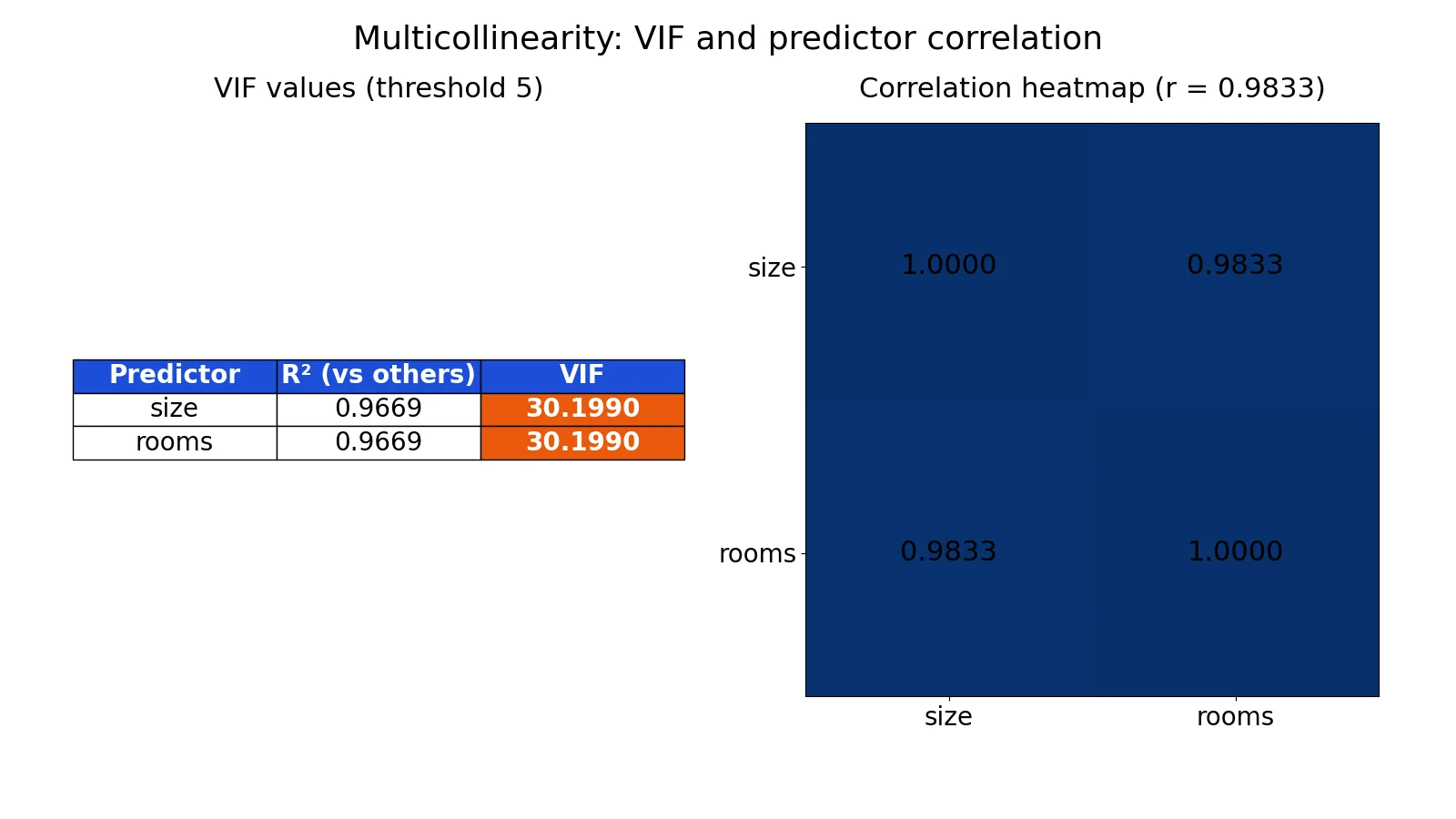
VIF(size)=30.1990, VIF(rooms)=30.1990

The figure below pairs the VIF table with a correlation heatmap.

Caption: Left: VIF table showing VIF(size)=30.1990 and VIF(rooms)=30.1990. Right: correlation heatmap with r=0.9833. Alt text: VIF table (size=30.20, rooms=30.20) and heatmap showing r=0.98 between size and rooms.

How to Interpret It

Read the VIF as a multiplier on the variance of a coefficient. A value of 1 means no inflation. Values between 1 and 5 are generally acceptable. Values above 5 deserve a look, and values above 10 usually indicate a serious problem. In the example, a VIF of 30.1990 means the coefficient variance is about 30 times what it would be with uncorrelated predictors.

The correlation between predictors gives you a quick first signal. A pairwise correlation of 0.9833 is very high, and it lines up with the large VIF. Correlation alone is not enough, though, because multicollinearity can involve three or more variables that are jointly dependent even when no single pair looks alarming. The VIF catches those cases because it regresses each predictor on all the others at once.

The key point for interpretation is that a high VIF does not mean the model predicts badly. It means you should not read the individual coefficients as clean, separate effects. If your goal is prediction, a high VIF may be tolerable. If your goal is to explain how each predictor affects the outcome, it is a real obstacle.

When to Use It (and when not to)

Use VIF and correlation checks whenever you fit a regression and plan to interpret the coefficients. This applies to linear models, and the same idea extends to related methods covered under multivariate analysis where several predictors enter at once. It matters most when predictors are naturally related, such as size and rooms, or height and weight.

You can worry less when prediction is the only goal and you do not care about individual coefficients. A model with high VIF can still forecast well. You can also relax when the correlated variables are control variables you are not trying to interpret.

Do not use VIF as a pass or fail gate on its own. It is a diagnostic, and the right response depends on your question. If you need to separate effects, consider dropping one predictor, combining them, or using a method designed for correlated inputs.

Multicollinearity vs Correlation

These two ideas are related but not the same. Correlation is a pairwise measure between two variables. Multicollinearity is a property of the whole predictor set and can involve many variables at once.

Aspect	Multicollinearity	Correlation
Scope	Whole set of predictors	Two variables at a time
Measure	VIF, condition number	Pearson r, Spearman, Kendall
Detects joint dependence	Yes	No
Example value	VIF = 30.1990	r = 0.9833
Effect on model	Inflates coefficient variance	A signal, not a full diagnosis

A high pairwise correlation often points to multicollinearity, but low pairwise correlations do not rule it out. That is why the VIF is the more complete check. For a deeper look at how two variables relate, see bivariate data.

Common Mistakes

Treating any correlation above 0.7 as fatal. Fix: check the VIF, because moderate pairwise correlation is often harmless.
Dropping a predictor just because its VIF is high. Fix: decide based on your research question, since dropping a variable can bias the remaining coefficients.
Ignoring multicollinearity because the model $R^2$ is high. Fix: remember that a high $R^2$ (0.9993 here) says nothing about coefficient stability.
Forgetting that categorical predictors can create dependencies. Fix: use sensible dummy coding and check the VIF after encoding [2].
Reading a sign flip as a real effect. Fix: treat unstable or nonsensical signs as a symptom of collinearity, not a finding [1].
Checking only pairwise correlations. Fix: run the full VIF, which catches joint dependence across three or more variables.

Limitations

VIF is a diagnostic, not a solution. It tells you that coefficients are unstable but does not tell you which variable to remove or how to fix the model. The thresholds of 5 and 10 are conventions, not laws, and the right cutoff depends on your context and sample size.

VIF also assumes you are working with a linear model and numeric predictors. It can mislead with interaction terms, polynomial terms, and some categorical setups, where high VIF values are expected and not necessarily a problem. Finally, multicollinearity is about the predictors only. It says nothing about whether your model is correctly specified or whether you have omitted important variables.

Frequently Asked Questions

What is a good VIF value?

A VIF of 1 means no inflation. Values below 5 are usually considered fine, and values above 10 are widely treated as a problem. These cutoffs are rules of thumb, so use them as guidance alongside your research goal.

Does multicollinearity affect prediction accuracy?

It affects the stability of individual coefficients more than overall predictions. A model with high VIF can still predict well, especially on new data drawn from the same population. The damage shows up when you try to interpret separate effects.

How do I fix multicollinearity?

Common fixes include removing one of the correlated predictors, combining them into a single index, or using a method built for correlated inputs such as ridge regression or principal component analysis [1]. The best choice depends on whether you need interpretation or just prediction.

Can multicollinearity make a coefficient negative when it should be positive?

Yes. When predictors overlap heavily, the model can assign a nonsensical sign to a coefficient, such as a negative value where common sense says positive [1]. This is one of the clearest warning signs that collinearity is distorting your estimates.

Is multicollinearity the same as correlation?

No. Correlation is a pairwise measure, while multicollinearity describes dependence across the whole predictor set. You can have multicollinearity with no single high pairwise correlation, which is why the VIF is the better check.