What Are Marginal Means? Definition and Examples

By Dr. Zubair Khalid, DVM, MS, PhD · 2026-10-03

Marginal means are the averages of the cell means in a row or column of a results table. They summarize how one factor behaves while collapsing over the other factors in the design. If you have ever looked at a two-way table of group averages and wondered what the numbers along the edges mean, those edge numbers are marginal means.

Quick Answer

A marginal mean is the mean of the cell means for one level of a factor, averaged across the levels of the other factor.
Cell means describe one specific combination, such as fertilizer = yes and light = low.
Marginal means collapse that combination down to a single factor, such as fertilizer = yes averaged over both light levels.
You compute them by averaging cell means, not by averaging the raw data points, when the design is balanced.
They appear in ANOVA output, in software menus, and in regression models as estimated marginal means [1][2].

What Marginal Means Mean

In plain language, a marginal mean is the average for one group when you ignore the other grouping variable. Suppose you run a study with two factors, fertilizer and light. You get four cell means, one for each combination. If you want to know how plants do with fertilizer overall, you average the two fertilizer = yes cell means. That single number is the marginal mean for fertilizer = yes.

The precise statistical definition is this. In a factorial design with factors A and B, the marginal mean for level $i$ of factor A is the mean of the cell means $\bar{Y}_{ij}$ across all levels $j$ of factor B:

$$\bar{Y}_{i\cdot} = \frac{1}{J}\sum_{j=1}^{J} \bar{Y}_{ij}$$

The dot in the subscript marks the factor that has been averaged over. So $\bar{Y}_{i\cdot}$ means "averaged over B." This is the same idea as a marginal distribution, where you sum or average over one variable to get the totals for the other. The word "marginal" comes from the old practice of writing these totals in the margins of a cross-tabulation table.

One important detail separates the simple version from the model-based version. When your design is balanced, the marginal mean is just the arithmetic average of the cell means. When the design is unbalanced, or when you fit a regression model with covariates, software reports estimated marginal means, which are model-based predictions averaged over the other factors [1]. The concept is the same, but the arithmetic is not.

How It Works

The mechanism is a two-step averaging process.

Step 1. Compute the cell means. For each combination of factor levels, take the mean of the observations in that cell.

$$\bar{Y}_{ij} = \frac{1}{n_{ij}}\sum_{k=1}^{n_{ij}} Y_{ijk}$$

Here $Y_{ijk}$ is the $k$-th observation in cell $(i,j)$, and $n_{ij}$ is the number of observations in that cell.

Step 2. Average across the other factor. For each level of the factor you care about, average the cell means.

$$\bar{Y}_{i\cdot} = \frac{1}{J}\sum_{j=1}^{J} \bar{Y}_{ij}$$

Each symbol means the following.

$i$ indexes the level of the factor you are summarizing, such as fertilizer = yes.
$j$ indexes the level of the factor you are collapsing over, such as light.
$J$ is the number of levels of that second factor.
$\bar{Y}_{ij}$ is the cell mean for combination $(i,j)$.
$\bar{Y}_{i\cdot}$ is the marginal mean for level $i$.

The grand mean is the average of all the marginal means, or equivalently the average of all cell means when the design is balanced.

$$\bar{Y}_{\cdot\cdot} = \frac{1}{I}\sum_{i=1}^{I}\bar{Y}_{i\cdot}$$

If every cell has the same number of observations, averaging cell means gives the same answer as averaging all the raw values. If the cells are unequal, the two approaches diverge, and that difference is one of the most common sources of confusion.

Worked Example

The dataset is a 2x2 plant growth study. Fertilizer (no or yes) is crossed with light (low or high), with 3 plants in each cell. Growth is measured in centimeters.

fertilizer	light	growth_cm
no	low	12.1
no	low	11.4
no	low	12.8
no	high	15.2
no	high	14.6
no	high	15.9
yes	low	18.3
yes	low	17.5
yes	low	19.1
yes	high	22.4
yes	high	21.7
yes	high	23.0

Step 1. Cell means.

No fertilizer, low light: mean of 12.1, 11.4, 12.8 = 12.1000
No fertilizer, high light: mean of 15.2, 14.6, 15.9 = 15.2333
Fertilizer, low light: mean of 18.3, 17.5, 19.1 = 18.3000
Fertilizer, high light: mean of 22.4, 21.7, 23.0 = 22.3667

Step 2. Marginal means.

Fertilizer = no: (12.1000 + 15.2333) / 2 = 13.6667
Fertilizer = yes: (18.3000 + 22.3667) / 2 = 20.3333
Light = low: (12.1000 + 18.3000) / 2 = 15.2000
Light = high: (15.2333 + 22.3667) / 2 = 18.8000

Step 3. Grand mean.

(13.6667 + 20.3333) / 2 = 17.0000

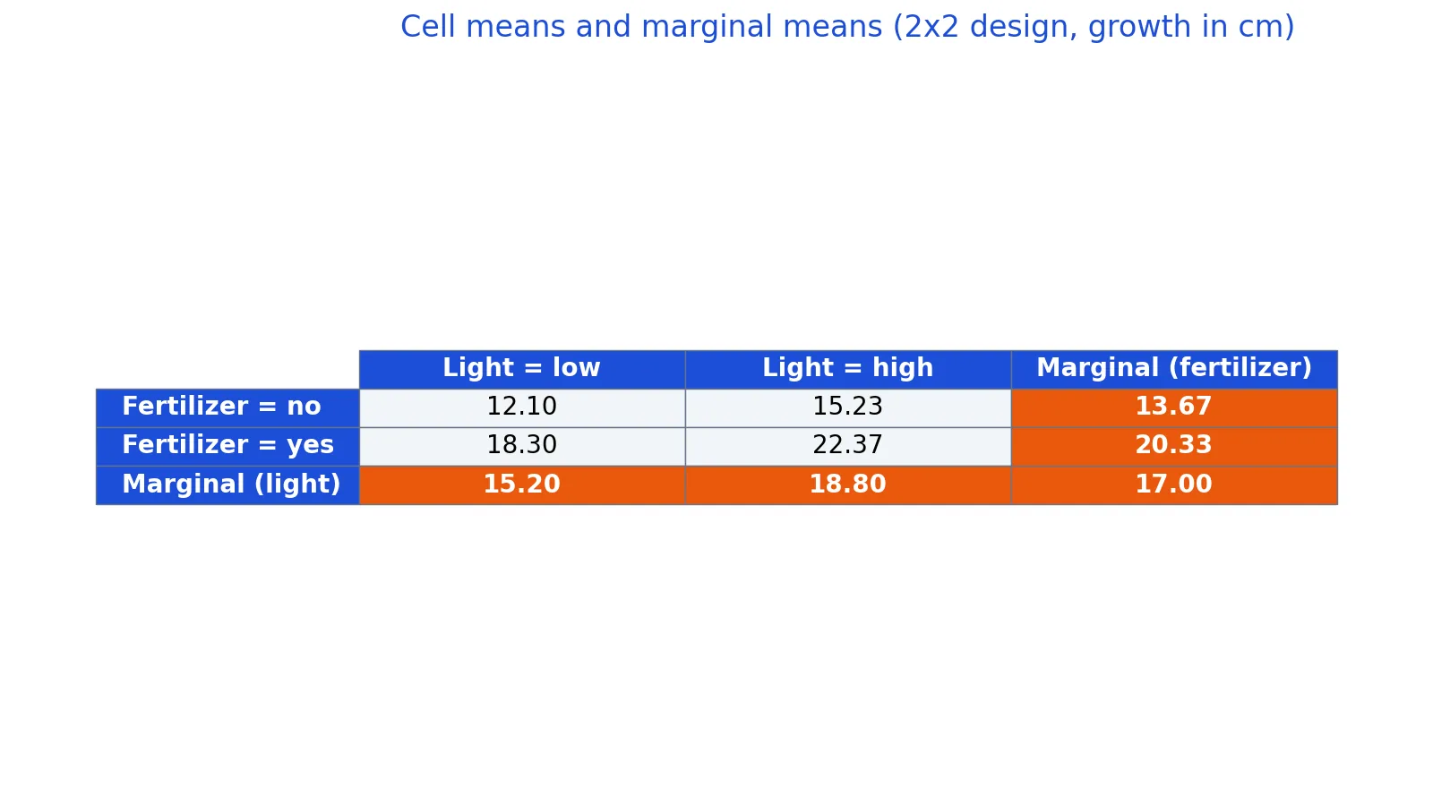
Table 1. Cell means and marginal means for the plant growth study.

	Light: low	Light: high	Marginal (fertilizer)
Fertilizer: no	12.10	15.23	13.67
Fertilizer: yes	18.30	22.37	20.33
Marginal (light)	15.20	18.80	17.00

The code below reproduces these numbers. It groups the raw data into cell means first, then averages those cell means by each factor.

import pandas as pd
df = pd.DataFrame({
    'fertilizer': ['no','no','no','no','no','no','yes','yes','yes','yes','yes','yes'],
    'light':      ['low','low','low','high','high','high','low','low','low','high','high','high'],
    'growth':     [12.1,11.4,12.8,15.2,14.6,15.9,18.3,17.5,19.1,22.4,21.7,23.0],
})
cell = df.groupby(['fertilizer','light'])['growth'].mean()
marg_fert  = cell.groupby('fertilizer').mean()
marg_light = cell.groupby('light').mean()
grand = cell.mean()
print(f"marginal_no={marg_fert['no']:.4f}, marginal_yes={marg_fert['yes']:.4f}, marginal_low={marg_light['low']:.4f}, marginal_high={marg_light['high']:.4f}, grand={grand:.4f}")

Output:

marginal_no=13.6667, marginal_yes=20.3333, marginal_low=15.2000, marginal_high=18.8000, grand=17.0000

How to Interpret It

Read a marginal mean as the average outcome for one level of a factor, averaged equally over the levels of the other factors. In the example, the marginal mean for fertilizer = yes is 20.33 cm. That is the average growth you would expect across both light conditions if you applied fertilizer.

Compare marginal means to the grand mean to see the size of a main effect. Fertilizer = no sits 3.33 cm below the grand mean of 17.00, and fertilizer = yes sits 3.33 cm above it. That symmetry is expected in a balanced design. The same logic applies to light, where low is 1.80 cm below the grand mean and high is 1.80 cm above.

Marginal means are also the numbers you plot when you want a clean visual of a main effect. A bar chart of the two fertilizer marginal means shows the overall fertilizer difference without the clutter of four separate cells. If you want a quick check on the arithmetic, a mean, median and mode calculator will confirm the raw averages for any single group.

When to Use It (and when not to)

Use marginal means when you want a single summary number per level of a factor, when you are reporting main effects from a factorial design, or when you need to compare groups while adjusting for an unbalanced design through a model [1]. They are the standard output for estimated marginal means in ANOVA workflows, and software such as jamovi exposes them directly in the post hoc settings [2].

Avoid relying on marginal means alone when an interaction is present. If the effect of fertilizer depends on light level, the marginal mean for fertilizer hides that pattern by averaging over it. In that case, report the cell means alongside the marginals. Also avoid treating a marginal mean as a description of any real subgroup. It may correspond to no actual group of subjects in your data.

Marginal Means vs Cell Means

Cell means and marginal means answer different questions. A cell mean describes one specific combination of factor levels. A marginal mean describes one level of a single factor, averaged over the others.

Feature	Cell mean	Marginal mean
Describes	One combination, such as no fertilizer and low light	One factor level, such as fertilizer = yes
Number of values in a 2x2 design	4	2 per factor, plus the grand mean
Sensitive to interactions	Yes, it shows them directly	No, it averages them away
Typical use	Detailed group comparisons	Main effects and summary reporting
Computed from	Raw observations in the cell	Cell means

If you want to see how one variable behaves on its own, ignoring the others, you are looking at a marginal view. That is the same logic behind a marginal distribution, which totals a contingency table along one axis.

Common Mistakes

Averaging raw data instead of cell means in an unbalanced design. When cell sizes differ, the mean of all raw values is not the same as the mean of the cell means. Fix: decide which quantity you want, then compute it deliberately. Most software reports the average of cell means for estimated marginal means.
Reading a marginal mean as a real subgroup. In this balanced example the marginal mean for fertilizer = yes happens to equal the mean of the six fertilized plants, but in an unbalanced design or a model with covariates it need not match any actual set of plants. Fix: describe it as an average across the other factor, not as a group.
Ignoring a significant interaction. Marginal means can look clean while the underlying cells tell a different story. Fix: always inspect cell means before interpreting main effects.
Confusing marginal means with marginal effects. A marginal mean is an average outcome. A marginal effect is a change in that outcome when a predictor changes [1]. Fix: check whether the number is a level or a difference.
Forgetting that model-based marginal means depend on the model. Estimated marginal means come from fitted predictions, so changing the model changes them. Fix: report the model and the averaging method you used.
Rounding cell means before averaging. Rounding 15.2333 to 15.23 before averaging shifts the marginal mean slightly. Fix: keep full precision through the calculation and round only the final result.

Limitations

Marginal means compress information. Any pattern that lives in the interaction between factors disappears once you average over one of them. Two datasets with identical marginal means can have completely different cell structures, so marginal means alone cannot tell you whether a factor behaves consistently across conditions.

The simple average-of-cell-means formula also assumes a balanced design. With unequal cell sizes, the arithmetic average of cell means weights each cell equally regardless of how many observations it contains, which may not match the population you care about. Model-based estimated marginal means handle this by averaging predicted values over a specified reference grid, but the answer then depends on the model and on which covariates you hold fixed [1]. Always state which version you are reporting.

Frequently Asked Questions

What is a marginal mean in simple terms?

A marginal mean is the average for one level of a factor after averaging over the other factors in the study. If you have a table of cell means, the marginal means are the row and column averages written along the edges.

How do marginal means differ from cell means?

A cell mean covers one exact combination of factor levels, such as no fertilizer with low light. A marginal mean covers one level of a single factor, such as fertilizer = yes, averaged across every level of the other factor.

Are marginal means the same as estimated marginal means?

They are closely related but not identical. A plain marginal mean is the arithmetic average of cell means in a balanced design. Estimated marginal means are model-based predictions averaged over a reference grid, which is what software reports for unbalanced designs and models with covariates [1].

Can I compute marginal means by hand?

Yes, for a balanced design. Compute each cell mean, then average the cell means across the factor you want to collapse. In the plant example, averaging 12.1000 and 15.2333 gives the marginal mean of 13.6667 for no fertilizer.

Why do marginal means sometimes look wrong?

The most common reason is an interaction. When one factor changes the effect of another, the marginal mean averages over that change and can describe a pattern that no subgroup actually shows. The second common reason is an unbalanced design, where the average of cell means differs from the average of raw observations.