Joint Frequency: Definition, Formula and Examples

By Dr. Zubair Khalid, DVM, MS, PhD · 2026-10-03

Joint frequency is the count of observations that fall into one specific combination of two categorical variables. In a two-way table, each interior cell holds one joint frequency, and dividing that count by the total number of observations gives the joint relative frequency. This article defines both terms, shows the formula, and works through a complete example.

Quick Answer

Joint frequency is the raw count in a single cell of a two-way table, for example the number of females who prefer product A.
Joint relative frequency is that count divided by the grand total, so it is a proportion between 0 and 1.
The formula is $\text{joint relative frequency} = \dfrac{\text{cell count}}{\text{grand total}}$.
Joint frequencies sit at the intersection of one row category and one column category, so they describe two variables at once.
All joint relative frequencies in a table sum to 1, which makes them easy to check.

What Joint Frequency Means

A joint frequency is the number of times two categories occur together in your data. If you survey people about gender and product preference, the count of females who prefer product A is one joint frequency. The count of males who prefer product B is another.

The precise statistical definition: given two categorical variables $X$ and $Y$, the joint frequency of the pair $(x_i, y_j)$ is the number of observations in the sample for which $X = x_i$ and $Y = y_j$ simultaneously. It is the entry in row $i$ and column $j$ of the two-way table, sometimes called a contingency table.

The word "joint" signals that you are looking at two variables at the same time. A marginal frequency, by contrast, is a row total or column total, and it describes only one variable. If you have not built the underlying table yet, start with a frequency table and then split one variable by another.

Joint relative frequency is the same idea expressed as a proportion. Instead of "32 respondents," you say "0.32 of the sample," which is 32 percent. Relative frequencies are easier to compare across studies with different sample sizes, which is why they appear so often in reports.

How It Works

The mechanics are simple. You build a two-way table, count the observations in each cell, then divide each cell by the grand total.

The joint frequency formula is just a count:

$$f_{ij} = \text{number of observations where } X = x_i \text{ and } Y = y_j$$

The joint relative frequency formula is:

$$r_{ij} = \frac{f_{ij}}{N}$$

Each symbol means the following:

$f_{ij}$ is the joint frequency in row $i$, column $j$.
$r_{ij}$ is the joint relative frequency for that same cell.
$N$ is the grand total, the sum of every cell in the table.
$x_i$ is the category of the first variable, such as Female.
$y_j$ is the category of the second variable, such as Prefer A.

Two structural facts follow from the definition. First, the row totals and column totals are marginal frequencies, and they are the sums of the joint frequencies along each row and column. Second, because every observation lands in exactly one cell, the joint frequencies sum to $N$ and the joint relative frequencies sum to 1.

Worked Example

The dataset is a survey of 100 respondents recording gender and product preference.

Gender	Prefer A	Prefer B	Row total
Female	32	18	50
Male	12	38	50
Column total	44	56	100

The grand total is $N = 100$. Now compute each joint frequency and its relative counterpart.

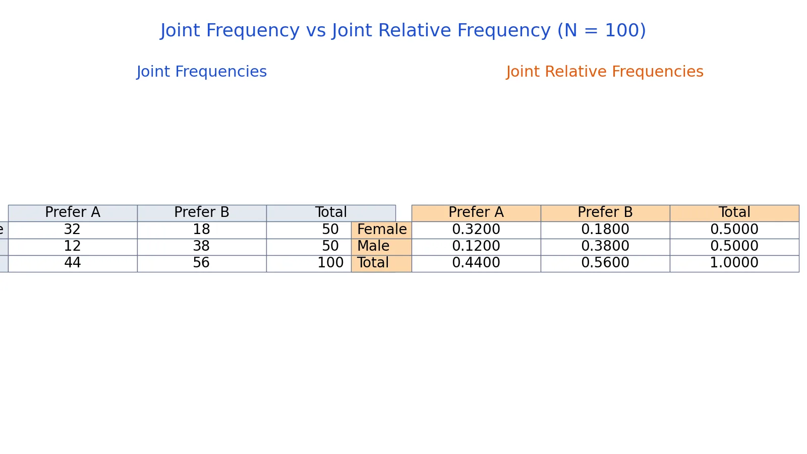
Female and Prefer A: count = 32, relative = 32 / 100 = 0.3200
Female and Prefer B: count = 18, relative = 18 / 100 = 0.1800
Male and Prefer A: count = 12, relative = 12 / 100 = 0.1200
Male and Prefer B: count = 38, relative = 38 / 100 = 0.3800

The row totals are 50 for Female and 50 for Male. The column totals are 44 for Prefer A and 56 for Prefer B. Adding the four relative frequencies gives 0.3200 + 0.1800 + 0.1200 + 0.3800 = 1.0000, which confirms the table is complete.

Here is the same computation in Python with pandas. The division broadcasts across the whole table at once.

import pandas as pd
df = pd.DataFrame(
    [[32, 18],
     [12, 38]],
    index=['Female','Male'],
    columns=['Prefer A','Prefer B'])
joint = df
joint_rel = df / df.values.sum()
print("joint_rel =")
print(joint_rel.to_string(float_format="%.4f"))

Output:

joint_rel =
          Prefer A  Prefer B
Female    0.3200    0.1800
Male      0.1200    0.3800

The left table holds joint frequencies, the right table holds joint relative frequencies. Both describe the same 100 respondents.

How to Interpret It

Read a joint frequency as a count of a specific subgroup. The value 32 means 32 respondents are both female and prefer product A. That is a concrete number you can report directly.

Read a joint relative frequency as a share of the whole sample. The value 0.3200 means 32 percent of all respondents are female and prefer product A. The denominator is always the grand total, never a row or column total.

That denominator is what separates joint relative frequency from conditional relative frequency. If you divided 32 by the Female row total of 50, you would get 0.64, the share of females who prefer A. That is a conditional relative frequency, and it answers a different question. Joint relative frequency describes the whole sample. Conditional relative frequency describes one subgroup.

A quick sanity check: the four joint relative frequencies must add to 1. If they do not, you have either miscounted a cell or used the wrong denominator.

When to Use It

Use joint frequency when you want to report raw counts of two-variable combinations, such as the number of customers in each region-product pair. Counts are useful when the total sample size matters, for example when you need to know whether a cell has enough observations to support a claim.

Use joint relative frequency when you want to compare patterns across tables with different totals, or when you want to describe the composition of a single sample. Proportions travel better than counts because they are scale-free.

Avoid joint frequencies when your two variables are measured on a continuous scale with many distinct values. A two-way table with hundreds of rows and columns becomes unreadable, and most cells will hold 0 or 1. In that situation, look at the relationship with a scatterplot or a covariance calculation instead.

Also avoid reading causation into any cell. A joint frequency tells you that two categories co-occur, not that one causes the other.

Joint Frequency vs Marginal Frequency

The closest related idea is marginal frequency, the row or column total. Marginal frequencies describe one variable on its own. Joint frequencies describe two variables together.

Feature	Joint frequency	Marginal frequency
What it counts	One row and one column category together	One category of a single variable
Position in table	Interior cell	Row total or column total
Example value	32 (Female and Prefer A)	50 (all females)
Relative version	Cell count / grand total	Row or column total / grand total
Sum of all values	Equals the grand total	Equals twice the grand total

The two are linked. Each marginal frequency is the sum of the joint frequencies in its row or column, so the interior cells carry all the information and the margins are derived from them.

Common Mistakes

Dividing by the row total instead of the grand total. That produces a conditional relative frequency, not a joint one. Fix it by always using $N$, the sum of every cell.
Confusing joint frequency with marginal frequency. A cell value of 32 is joint, a row total of 50 is marginal. Check the position in the table before labeling the number.
Forgetting to verify the totals. If the joint relative frequencies do not sum to 1, a cell was miscounted. Add them as a routine check.
Reporting a proportion as a percentage without converting. A value of 0.3200 is 32 percent, not 0.32 percent. Multiply by 100 when you write it as a percentage.
Treating a small cell count as reliable. A joint frequency of 2 or 3 supports very little. Note the count alongside the proportion so readers can judge.
Assuming the table is complete when categories overlap. Each observation must fall in exactly one row and one column. Overlapping categories break the sum-to-1 property.

Limitations

Joint frequencies describe association, not causation. A large cell tells you two categories appear together often, but it says nothing about why. You need a designed study or further analysis to make a causal claim.

The method also depends on how you define your categories. Collapsing or splitting a category changes every cell in the table, so two analysts can produce different joint frequencies from the same raw data. Report your category definitions alongside the table.

Finally, joint relative frequencies hide sample size. A proportion of 0.32 from 100 respondents and a proportion of 0.32 from 10 respondents look identical in a relative table but carry very different weight. Always keep the counts visible, or report both tables side by side.

Frequently Asked Questions

What is joint frequency in simple terms?

Joint frequency is the count of observations that share two specific characteristics at once. In a two-way table, it is the number sitting in one interior cell, at the crossing of one row category and one column category. The word "joint" refers to the two variables being considered together.

How do you calculate joint relative frequency?

Divide the joint frequency in a cell by the grand total of the table. If 32 respondents are female and prefer product A out of 100 total, the joint relative frequency is 32 / 100 = 0.32. Repeat for every cell, and the results will sum to 1.

What is the difference between joint and marginal frequency?

A joint frequency counts one combination of two variables, such as Female and Prefer A. A marginal frequency counts one variable alone, such as all females or all respondents who prefer A. Marginal frequencies are the row and column totals, and each one equals the sum of the joint frequencies in its row or column.

Do joint relative frequencies always add up to 1?

Yes, when the categories are mutually exclusive and cover every observation. Each respondent falls into exactly one cell, so the proportions partition the whole sample. If your values do not sum to 1, check for overlapping categories, missing data, or a counting error.

Can joint frequency be used with more than two variables?

A standard two-way table handles two variables. With three or more, you can build separate tables for each level of the extra variable, or use a multi-way contingency table. The same counting logic applies, but the table becomes harder to read as dimensions grow, so consider a frequency distribution or a modeling approach instead.

References

This article draws on the standard references listed under Further Reading.