How to Find a Circular Reference in Excel (Step by Step)

By Dr. Zubair Khalid, DVM, MS, PhD · 2026-10-03

If Excel shows a circular reference warning, or a formula suddenly returns 0, one cell is pointing back at itself, directly or indirectly. The fastest way to find a circular reference in Excel is to open the Circular References list under Formulas > Error Checking, then trace each listed cell. This guide walks through the whole process, from the first warning to a clean workbook.

Quick Answer

A circular reference happens when a formula refers to its own cell, either directly or through a chain of other cells [1].
Go to Formulas > Error Checking > Circular References to see a list of the cells involved [1].
Select each listed cell and check its formula for a reference that points back to itself [1].
Use Formulas > Trace Precedents or Trace Dependents to follow the loop when it spans several cells [1].
Repeat until the status bar no longer shows Circular References [1].

Before You Start

Two things are worth checking first, because they change what you see.

Excel shows a warning dialog the first time a circular reference appears in a session. Later circular references in the same session might not trigger the same dialog, so you cannot rely on the popup alone [1]. Watch the status bar instead. It can display "Circular References" plus one cell address. If the circular reference sits on another worksheet, you might only see "Circular References" with no address [1].

Also confirm that automatic calculation is on. Go to the Calculation options section, under Workbook Calculation, and make sure Automatic is selected [2]. With manual calculation, values can look stale and you may misread a circular reference as a wrong answer.

One more note before you dig in. In browser-based workbooks, a formula with an unresolvable circular reference does not show a warning at all. It calculates the values you would get if you canceled the operation on the Excel desktop client, which effectively cancels the circular reference automatically [3]. If you are working in the browser, open the file in the desktop app to see the real problem.

Step by Step

Look at the status bar. If it reads "Circular References" with a cell address, that address is your starting point [1]. If it shows no address, the loop is likely on another sheet [1].

Open the Circular References list. Go to Formulas > Error Checking > Circular References [1]. Excel lists the cells it has flagged.

Select the first listed cell. Read its formula in the formula bar. Look for a reference to the cell itself, like =D1+D2+D3 sitting in D3 [1].

Trace the chain if the loop is indirect. Select the cell and use Formulas > Trace Precedents to see which cells feed into it, or Formulas > Trace Dependents to see which cells it feeds [1]. Follow the arrows until they lead back to where you started.

Fix the formula. Change the reference so it no longer points back to its own cell. The fix is either to move the formula to another cell or to rewrite the syntax so it avoids the circular reference [2].

Clear the arrows. Once you have identified the offending cell, go to the Formula Auditing group on the Formulas tab and click Remove Arrows [4].

Check the status bar again. Repeat the steps until "Circular References" no longer appears [1].

If you are still building out the sheet, it helps to know how Excel reads references before you edit. Our guide on absolute reference in Excel explains when a reference locks to a cell and when it shifts, which is often the root of an accidental loop.

Worked Example

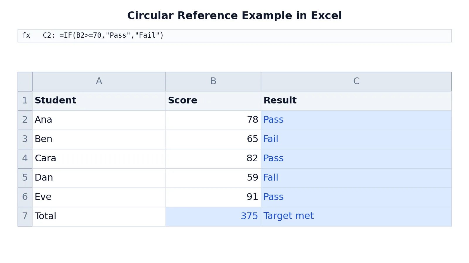
Here is a small score sheet. Column C holds Pass or Fail formulas, B7 totals the scores, and C7 compares that total to a target.

	A	B	C
1	Student	Score	Result
2	Ana	78	`=IF(B2>=70,"Pass","Fail")` -> displays Pass
3	Ben	65	`=IF(B3>=70,"Pass","Fail")` -> displays Fail
4	Cara	82	`=IF(B4>=70,"Pass","Fail")` -> displays Pass
5	Dan	59	`=IF(B5>=70,"Pass","Fail")` -> displays Fail
6	Eve	91	`=IF(B6>=70,"Pass","Fail")` -> displays Pass
7	Total	`=SUM(B2:B6)` -> displays 375	`=IF(B7>=350,"Target met","Below target")` -> displays Target met

Each result cell checks one score and returns a label:

C2 checks Ana's score and returns Pass or Fail.
C3 checks Ben's score and returns Pass or Fail.
C4 checks Cara's score and returns Pass or Fail.
C5 checks Dan's score and returns Pass or Fail.
C6 checks Eve's score and returns Pass or Fail.
B7 sums the scores in B2:B6 and returns 375.
C7 compares the total to the target and returns a status.

Now suppose someone edits C7 to read =IF(C7>=350,"Target met","Below target"). The formula now refers to its own cell, so Excel cannot finish the calculation [1]. The status bar shows Circular References, and the Circular References list points at C7. The fix is to restore the reference to B7, the cell that actually holds the total. Once you do, C7 returns "Target met" again because 375 is greater than or equal to 350.

This is the most common shape of the problem. A formula that should read from a neighbor accidentally reads from itself, and the value collapses to 0 or a warning.

Other Ways to Do It

The Circular References list is the primary tool, but a few others help when the loop is hard to see.

Go To for a known address. If the status bar gives you a cell address, press Ctrl+G on Windows or Control+G on Mac to jump straight to it [1]. You can also type a sheet-qualified reference such as sheet2!$D$12 in the Reference box to reach a cell on another sheet [5].

Go To Special for formulas. If you suspect a whole region is affected, click Home > Find & Select > Go To Special, then click Formulas to select every formula cell in the sheet or in your selected range [6]. This narrows the search to cells that can actually contain a loop.

Trace arrows for the chain. Trace Precedents and Trace Dependents draw arrows between related cells, which makes an indirect loop visible [1]. Remove Arrows clears them when you are done [4].

If your sheet is large and you are hunting for other kinds of problems at the same time, the techniques in how to find and search in Excel speed up the scan.

Troubleshooting

The status bar shows Circular References but no address. The loop is probably on another worksheet [1]. Check each sheet, or use Go To Special on each one to list formula cells.

Error Checking or Circular References is grayed out. These commands vary by platform and build [1]. On Windows desktop and Mac desktop, the path is Formulas > Error Checking > Circular References [1]. If the command is unavailable in your build, fall back to Go To Special and manual tracing.

The warning dialog never appeared. Excel shows the warning only the first time a circular reference is created in a session. Later ones might not trigger the same dialog [1]. Trust the status bar over the popup.

You fixed one cell and another appears. Circular references often come in groups. Keep working through the list and recheck the status bar after each fix [1].

The value is 0 and you cannot see why. A formula that refers to its own cell cannot be calculated, so the result is not meaningful [7]. Trace precedents from the zero cell to find the loop.

Common Mistakes

Editing the wrong cell in the loop. The Circular References list may show several cells. Fix the one whose formula actually points back at itself, not the first address you see. Use Trace Precedents to confirm.
Deleting the formula instead of fixing it. Deleting removes the error but also removes the calculation. Rewrite the reference so it points to the correct cell [2].
Turning on iterative calculation to hide the problem. Iteration lets Excel recalculate a circular formula repeatedly until a numeric condition is met [7]. That is a deliberate modeling choice, not a cleanup step. If you enable it by accident, the loop stays in the workbook.
Ignoring the browser. A browser-based workbook silently cancels an unresolvable circular reference instead of warning you [3]. Open the file in the desktop app before you conclude the sheet is clean.
Leaving tracer arrows on. Arrows pile up and clutter the sheet. Click Remove Arrows once you have found the cell [4].
Assuming the popup is the only signal. After the first warning in a session, later circular references may not show a dialog [1]. Check the status bar every time.

Limitations

The Circular References list shows cells Excel has flagged, and the status bar may show only one address even when several loops exist [1]. It does not explain why the loop exists or which reference to change. You still have to read the formulas and decide.

Trace arrows also stop being useful in very large or heavily linked workbooks, where the arrows overlap and the chain is hard to follow. And in browser-based workbooks, the warning behavior differs entirely, so the desktop tools are the reliable ones [3]. If you need a formula to iterate on purpose, that is a separate setting with its own controls for maximum iterations and maximum change [7].

Frequently Asked Questions

How do I find a circular reference in Excel quickly?

Open Formulas > Error Checking > Circular References and select each listed cell [1]. Read the formula in the formula bar and look for a reference to the cell itself. If the loop is indirect, use Trace Precedents or Trace Dependents to follow the chain [1].

Why does my formula return 0 instead of a value?

A formula that refers to its own cell cannot be calculated, so Excel cannot produce a meaningful result [7]. The zero is a symptom, not an answer. Find the self-reference and correct it.

How do I remove circular references in Excel?

Fix each flagged formula so it no longer points back to its own cell, then recheck the status bar [1]. Repeat until "Circular References" disappears. If you genuinely need the loop to iterate, enable iterative calculation instead, which lets Excel recalculate the formula a set number of times [7].

Can a circular reference be intentional?

Yes. Iteration is the repeated recalculation of a worksheet until a specific numeric condition is met, and circular references can be used that way on purpose [7]. You control the maximum number of iterations and the acceptable amount of change [7]. Solver and Goal Seek also use iteration in a controlled way [7].

Why does the status bar show Circular References with no cell address?

That usually means the circular reference is on another worksheet [1]. Check each sheet in turn, or use Go To Special to list formula cells on each one [6]. Once you find the loop, the address will appear normally.

If you want to rebuild the sheet from scratch with clean formulas, start with how to make a formula in Excel and how to sum a column in Excel. Both cover the reference patterns that prevent loops before they start.