How to Find Duplicates in Excel (Step by Step)
By Dr. Zubair Khalid, DVM, MS, PhD ·
To find duplicates in Excel, you can use conditional formatting to highlight them, a COUNTIF formula to count and label them, or the Remove Duplicates tool to delete them. Each method answers a slightly different question, so the right choice depends on whether you want to see the duplicates, count them, or remove them.
Quick Answer
- Highlight duplicates visually: Select your range, then go to Home > Conditional Formatting > Highlight Cells Rules > Duplicate Values [1].
- Count and label duplicates: Use
=COUNTIF($A$2:$A$13,A2)in a helper column, then wrap it in=IF(B2>1,"Duplicate","Unique"). - Remove duplicates permanently: Select your data, then go to Data > Remove Duplicates and choose which columns to check [1].
- Check before deleting: Copy your original data to another worksheet first, because Remove Duplicates deletes data permanently [1].
- Google Sheets: Use Format > Conditional formatting with a custom formula like
=COUNTIF($A$2:$A$13,A2)>1.
Before You Start
Duplicate detection works best when your data is clean and consistently formatted. A few preparation steps save time later.
First, decide what counts as a duplicate. In a customer list, two rows with the same Customer ID are duplicates even if the names differ. In a sales table, a duplicate might mean the same order number appears twice. Define the key column or column combination before you start.
Second, remove any outlines or subtotals from your data before using Remove Duplicates [1]. Outlines and subtotals change the row structure and can cause the tool to behave unexpectedly.
Third, check for hidden inconsistencies. Excel treats "CUST-1001" and "cust-1001 " as different values because of the trailing space. COUNTIF, Duplicate Values highlighting and Remove Duplicates all ignore case, so the case difference alone would not stop a match. The counts reported after removal can include empty cells and spaces, so trim your data first if accuracy matters [1].
Fourth, back up your sheet. Remove Duplicates deletes rows permanently, so copy the original data to another worksheet before you run it [1].
If you want to explore related cleanup tasks, see how to remove duplicates in Excel once you have identified them.
Step by Step
These steps use a formula-based approach that works in every modern version of Excel and gives you a permanent, auditable record of which rows are duplicates.
- Select the column you want to check. Click the column header or select the exact range, for example A2:A13.
- Add a helper column next to your data. In B1, type a label such as
COUNTIF. In C1, typeDuplicate?.
- Enter the COUNTIF formula in B2. Type
=COUNTIF($A$2:$A$13,A2). The dollar signs lock the range so it does not shift when you copy the formula down.
- Enter the label formula in C2. Type
=IF(B2>1,"Duplicate","Unique"). This converts the raw count into a readable flag.
- Copy both formulas down. Select B2:C2, then drag the fill handle down to row 13. Each row now shows how many times its value appears and whether it is a duplicate.
- Filter or sort by the Duplicate? column. Use Data > Filter to show only rows marked Duplicate. This is the fastest way to review them before deciding what to do.
- Optionally highlight duplicates with color. Select A2:A13, then go to Home > Conditional Formatting > Highlight Cells Rules > Duplicate Values. Pick a fill color and click OK [1].
- Remove duplicates only when you are ready. Select A1:C13, then go to Data > Remove Duplicates. In the dialog, check My data has headers, tick Customer ID, and click OK [1].
If you need to search for a specific value before flagging duplicates, the techniques in how to find and search in Excel cover that.
Worked Example
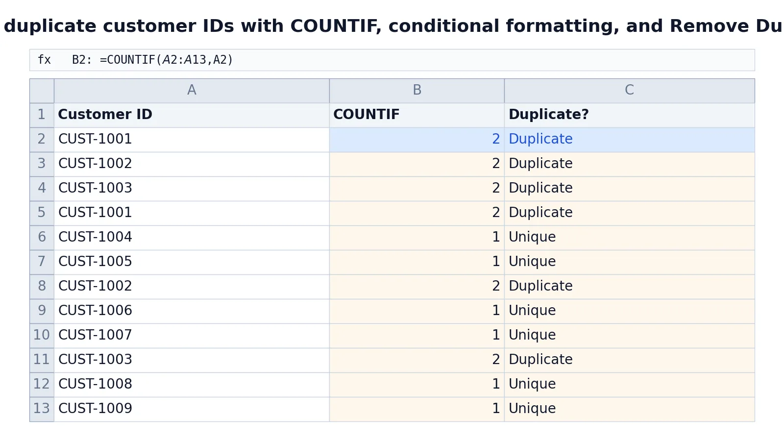
This example uses a 12-row customer ID list in column A, with a COUNTIF helper column in B and a Duplicate? label in column C.
| Row | A | B | C |
|---|---|---|---|
| 1 | Customer ID | COUNTIF | Duplicate? |
| 2 | CUST-1001 | =COUNTIF($A$2:$A$13,A2) -> 2 | =IF(B2>1,"Duplicate","Unique") -> Duplicate |
| 3 | CUST-1002 | =COUNTIF($A$2:$A$13,A3) -> 2 | =IF(B3>1,"Duplicate","Unique") -> Duplicate |
| 4 | CUST-1003 | =COUNTIF($A$2:$A$13,A4) -> 2 | =IF(B4>1,"Duplicate","Unique") -> Duplicate |
| 5 | CUST-1001 | =COUNTIF($A$2:$A$13,A5) -> 2 | =IF(B5>1,"Duplicate","Unique") -> Duplicate |
| 6 | CUST-1004 | =COUNTIF($A$2:$A$13,A6) -> 1 | =IF(B6>1,"Duplicate","Unique") -> Unique |
| 7 | CUST-1005 | =COUNTIF($A$2:$A$13,A7) -> 1 | =IF(B7>1,"Duplicate","Unique") -> Unique |
| 8 | CUST-1002 | =COUNTIF($A$2:$A$13,A8) -> 2 | =IF(B8>1,"Duplicate","Unique") -> Duplicate |
| 9 | CUST-1006 | =COUNTIF($A$2:$A$13,A9) -> 1 | =IF(B9>1,"Duplicate","Unique") -> Unique |
| 10 | CUST-1007 | =COUNTIF($A$2:$A$13,A10) -> 1 | =IF(B10>1,"Duplicate","Unique") -> Unique |
| 11 | CUST-1003 | =COUNTIF($A$2:$A$13,A11) -> 2 | =IF(B11>1,"Duplicate","Unique") -> Duplicate |
| 12 | CUST-1008 | =COUNTIF($A$2:$A$13,A12) -> 1 | =IF(B12>1,"Duplicate","Unique") -> Unique |
| 13 | CUST-1009 | =COUNTIF($A$2:$A$13,A13) -> 1 | =IF(B13>1,"Duplicate","Unique") -> Unique |
The COUNTIF in B2 counts how many times the Customer ID in A2 appears in the whole list. A count above 1 means it is repeated. The IF formula in C2 turns that count into a readable label: Duplicate when the count is greater than 1, otherwise Unique.
In this dataset, three IDs repeat: CUST-1001, CUST-1002, and CUST-1003. Each appears twice, so each row carrying one of those IDs shows a count of 2 and the label Duplicate. The remaining six IDs appear once and are labeled Unique.
The formula logic in plain terms:
$$ \text{COUNTIF}(A2:A13, A2) > 1 \Rightarrow \text{Duplicate} $$
To apply the same logic visually, select A2:A13, then go to Home > Conditional Formatting > Highlight Cells Rules > Duplicate Values. In the Duplicate Values dialog, choose a highlight color and click OK. To delete the repeats instead, select A1:C13, then go to Data > Remove Duplicates. In the Remove Duplicates dialog, check My data has headers, tick Customer ID, and click OK [1].
Other Ways to Do It
Conditional formatting alone. If you only need to see duplicates, skip the helper columns. Select your range and apply Home > Conditional Formatting > Highlight Cells Rules > Duplicate Values [1]. This is the fastest visual check. Note that Excel cannot highlight duplicates in the Values area of a PivotTable report [1].
Remove Duplicates. This tool deletes repeated rows permanently. Select your range, go to Data > Remove Duplicates, and check or uncheck the columns you want to compare [1]. If you have a January price column you want to keep, uncheck January in the dialog so it is not used in the comparison [1].
Filter and sort. Sorting your data alphabetically or numerically groups identical values together, which makes duplicates easy to spot by eye. Combine this with the filter in Excel feature to isolate specific values.
Google Sheets. Select your range, then go to Format > Conditional formatting. Choose Custom formula is and enter =COUNTIF($A$2:$A$13,A2)>1. Pick a fill color and click Done. To delete repeats in Google Sheets, use the built-in Data > Data cleanup > Remove duplicates option.
Count unique values instead. If you want to know how many distinct values exist, see how to count unique values in Excel.
Troubleshooting
The COUNTIF returns 1 for a value you can see repeated. Check for trailing spaces or non-printing characters. Use =TRIM(A2) in a helper column to clean the text, then run COUNTIF against the cleaned column.
Conditional formatting highlights nothing. Confirm your range is selected correctly and that the rule applies to the right cells. Also check whether the cells are in a PivotTable Values area, where duplicate highlighting does not work [1].
Remove Duplicates removes more rows than expected. The tool compares all checked columns. Rows that match in all checked columns are treated as duplicates, so if you uncheck a column that should be part of the comparison, rows that differ only in that column are removed. Check every column that defines a duplicate [1].
The duplicate count includes blanks. Counts reported after removal can include empty cells and spaces [1]. Filter out blanks before running your check.
Formulas break when you insert rows. Absolute references like $A$2:$A$13 do not expand automatically. If you add rows, update the range or convert your data to an Excel Table so ranges adjust automatically.
Common Mistakes
- Deleting before reviewing. Remove Duplicates deletes data permanently. Copy your original data to another worksheet first [1].
- Checking the wrong columns. If you leave a column checked that should not be part of the comparison, you get the wrong duplicate set. Uncheck columns like January when they hold values you want to keep [1].
- Ignoring case and spaces. Excel treats "CUST-1001" and "cust-1001 " as different. Trim and standardize your text before checking.
- Using relative references in COUNTIF. Without dollar signs, the range shifts as you copy down and your counts become wrong. Use
$A$2:$A$13. - Forgetting outlines and subtotals. Remove outlines or subtotals before using Remove Duplicates, or the tool may behave unexpectedly [1].
- Assuming conditional formatting removes data. Highlighting only changes appearance. The underlying rows stay in place until you delete them.
Limitations
Formula-based duplicate detection works on exact matches. It cannot find near-duplicates such as "John Smith" and "Jon Smith" unless you build fuzzy matching logic yourself. It also treats text as case-insensitive in COUNTIF, so "ABC" and "abc" count as the same value, which may or may not match your intent.
Conditional formatting and Remove Duplicates both operate on the range you select. If your data spans multiple sheets or workbooks, you need to consolidate it first or run the check separately on each sheet. Neither method understands relationships between columns beyond exact value matching, so a duplicate order number with a different customer name will still be flagged as a duplicate if you only check the order number column.
Frequently Asked Questions
How do I find duplicates in Excel without deleting them?
Use conditional formatting or a COUNTIF helper column. Select your range, then go to Home > Conditional Formatting > Highlight Cells Rules > Duplicate Values to color the repeats [1]. Alternatively, enter =COUNTIF($A$2:$A$13,A2) in a helper column and filter for values greater than 1. Both methods leave your original data untouched.
How do I check duplicates in Excel across two columns?
Use =COUNTIF($B$2:$B$100,A2) to check whether each value in column A also appears in column B. A result greater than 0 means the value exists in both columns. For a full row comparison, concatenate the columns with =A2&B2 and run COUNTIF on the combined values.
How do I find duplicates in Google Sheets?
Select your range, then go to Format > Conditional formatting. Choose Custom formula is and enter =COUNTIF($A$2:$A$13,A2)>1. Pick a fill color and click Done. Google Sheets highlights every cell whose value appears more than once in the range.
Why does Remove Duplicates delete rows I wanted to keep?
Remove Duplicates compares every checked column. If two rows match in all checked columns, one is deleted. To protect a column like January price data, uncheck it in the Remove Duplicates dialog so it is excluded from the comparison [1]. Always copy your data first because the deletion is permanent [1].
Can Excel highlight duplicates in a PivotTable?
No. Excel cannot highlight duplicates in the Values area of a PivotTable report [1]. If you need to flag duplicates in summarized data, copy the PivotTable values to a regular range first, then apply conditional formatting to that range.
References
Further Reading
- Broman KW, Woo KH (2018). Data Organization in Spreadsheets. The American Statistician
- Ziemann M, Eren Y, El-Osta A (2016). Gene name errors are widespread in the scientific literature. Genome Biology
- Microsoft Support: Excel help and learning
- McCullough B, Heiser DA (2008). On the accuracy of statistical procedures in Microsoft Excel 2007. Computational Statistics & Data Analysis
- Abeysooriya M, Soria M, Kasu MS et al. (2021). Gene name errors: Lessons not learned. PLOS Computational Biology